2 Fundamental concepts

2.1 A Stochastic Point of View

The observed time series \(\rnd X_1, \dots,\rnd X_n\) is a sequence of numbers and our aim is to understand the mechanism that generated the series and make use of it. Therefore we need a mathematical model, then capture randomness, by which we mean a model for uncertainty and/or limited knowledge. Partial information also will need to be addressed. The observed data are seen as a sequence of realizations of random variables and as such we need to study them all together, including their relationships.

Definition 2.1 A stochastic process is a family of random variables \(\set{\rnd X_t : t \in T}\) defined on a probability space \((\Omega, \mcal{A}, P)\).

Where in the Definition 2.1 the meaning of used symbols is as follows:

\(T\) is the index set;
\(\set{\rnd X_t : t \in T}\) can be seen as a function of \(t\) and \(\omega\), i.e., \(\set{\rnd X (t, \omega) : t \in T, \omega \in \Omega}\);
for a fixed \(t \in T, \; \rnd X_t = \rnd X_t (\cdot) = \set{\rnd X_t (\omega) : \omega \in \Omega}\) is a random variable defined on \(\Omega\), i.e. the process is seen as a collection of random variables indexed by \(T\);
for a fixed \(\omega \in \Omega, \; \rnd X = \rnd X(\omega) = \set{\rnd X_t (\omega) : t \in T}\) is a function on \(T\), i.e. the process is seen as a random function.

As such, we call a realization of \(\set{\rnd X_t : t \in T}\) a sample path/trajectory/realization.

2.1.1 Types of stochastic processes

There are many types of stochastic processes, but most importantly (for us):

time series (discrete-time processes)
- \(T = \Z\) (or \(T \subset \Z\), e.g., \(T = \N\));
- the observed time series is seen as a realization of the stochastic process \(\set{\rnd X_t : t \in \Z} = \set{\dots , \rnd X_{-1}, \rnd X_0, \rnd X_1, \dots}\);
- a time series is a random sequence and a sequence of random variables;
continuous-time processes: \(T = \R\) or \(T = [a, b]\) (random function);
spatially indexed processes: \(T = \R^d\) or \(T \subset \R^d\) (random fields);
processes on lattices: \(T = \Z^d, \dots\);
spatio-temporal processes: \(T = \R^d \times [a, b], \dots\);
etc.

Although we will see other types of index sets in other courses, in our lectures we will stick to time series only (where time is discretized).

2.1.2 Discrete sampling of time series

Time series are random sequences, i.e., \(T = \Z\), where the discretization can be due to discrete sampling of a continuous-time process, e.g. closing prices of a share, electrical signal in telecommunications, aggregation of a continuous time process, e.g. daily precipitation, monthly electricity production, or a discrete realization, e.g. regularly repeated medical experiment.

2.2 Distribution of a stochastic process

We can define a finite-dimensional distributions for all \(k \in \N, t_1, \dots, t_k \in T\) as \[ F_{t_1,\dots,t_k} (x_1, \dots, x_k) = P(\rnd X_{t_1} \leq x_1, \dots, \rnd X_{t_k} \leq x_k). \]

Here, we took a random vector \(\rnd X_{t_1}, \dots, \rnd X_{t_k}\) and looked at its joint distribution.

A system of distribution functions \(\set{F_{t_1, \dots, t_k}: \; t_1, \dots, t_k \in T, k \in \N}\) is called consistent, if it has following properties

\(\lim_{x_{k+1} \to \infty} F_{t_1, \dots, t_k, t_{k+1}}(x_1, \dots, x_k, x_{k+1}) = F_{t_1, \dots, t_k}(x_1, \dots, x_k)\);
\(F_{t_1, \dots, t_k}(x_1, \dots, x_k) = F_{t_{i_1}, \dots, t_{i_k}}(x_{i_1}, \dots, x_{i_k})\) for all permutations \((i_1, \dots, i_k)\) of \((1, \dots, k)\).

A stochastic process has always a consistent system of distributions.

Theorem 2.1 (Daniell–Kolmogorov) Let \(\set{ F_{t_1,\dots,t_k} : t_1,\dots, t_k \in T , k \in \N}\) be a consistent system of distribution functions. Then there exists a stochastic process \(\set{\rnd X_t : t \in T}\) such that for all \(k \in \N, t_1, \dots, t_k \in T\) the joint distribution function of \((X_{t_1} , \dots, X_{t_k})\) is \(F_{t_1, \dots,t_k}\).

For the distribution of a stochastic process, it holds that a process whose finite-dimensional distributions are all multivariate normal is called Gaussian. Often, much information is contained in means, variances and covariances and thus, focusing on the first and second moments is often sufficient. Moreover, if the joint distributions are multivariate normal, the first and second moments completely determine the joint distribution

Definition 2.2 (Mean, autocovariance, autocorrelation) For a stochastic process, we define:

mean function \[ \procMean_t = \expect \rnd X_t , t \in \Z; \]
autocovariance function (acov) \[ \acov(s, t) = \cov (\rnd X_s , \rnd X_t) = \Expect{(\rnd X_s − \procMean_s )(\rnd X_t − \procMean_t)}, \; s, t \in \Z; \]
autocorrelation function (acf) \[ \acf(s, t) = \corr (\rnd X_s ,\rnd X_t) = \frac{\cov (\rnd X_s, \rnd X_t)} {\sqrt{\variance \rnd X_s \variance \rnd X_t}} , \; s, t \in \Z. \]

2.3 Examples

2.3.1 White noise process

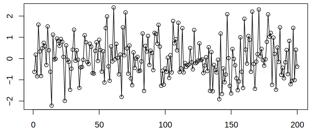
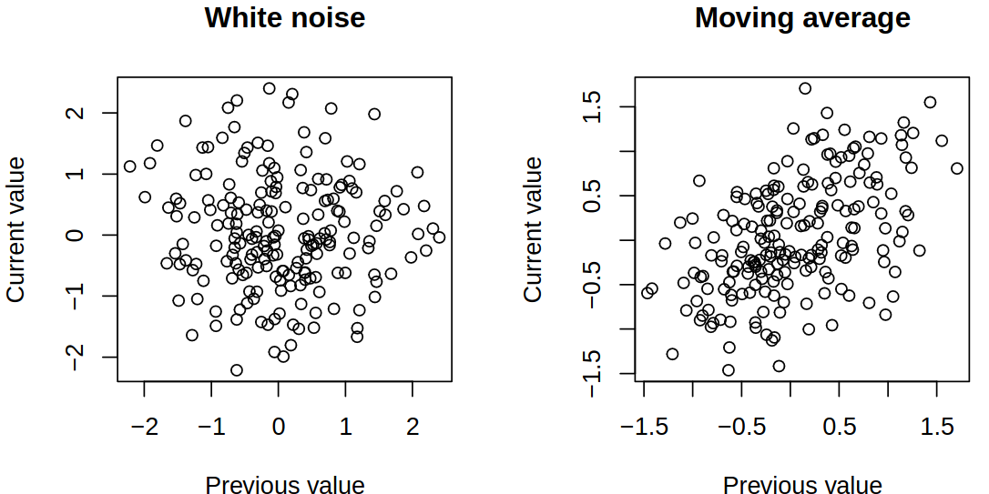
Let \(\set{\rve_t : t \in \Z}\) be a sequence of uncorrelated random variables with mean \(0\) and variance \(\procVar\). That is, \(\expect{\rnd X_t} = 0, \variance \rnd X_t = \procVar\), \(\cov(\rnd X_s , \rnd X_t) = 0, s \neq t\) and we introduce notation \(\set{\rve_t} \sim \WN{0}{\procVar}\).

2.3.2 Moving average

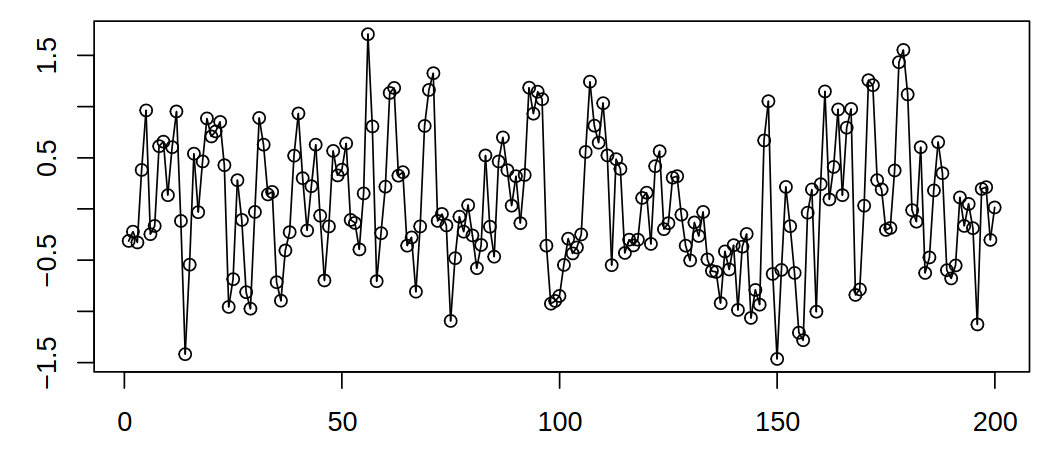
Let \(\set{\rve_t : t \in \Z}\) be \(\WN{0}{\procVar}\) and define \[ \rnd X_t = (\rve_{t} + \rve_{t-1})/2. \]

Then the mean function is given by \[ \procMean_t = \Expect{\rve_t +\rve_{t-1}}/2 = 0, \] and the variance by \[ \acov(t,t) = \Variance{(\rve_t + \rve_{t-1})/2} = \frac {\procVar} 2. \] Then autocovariance of the process is \[ \begin{gathered} \acov(t, t+1) = \cov \brackets{(\rve_t + \rve_{t-1})/2, (\rve_{t+1} + \rve_t)/2} = \frac{\procVar} 2, \\ \acov(t, t+h) = \cov \brackets{(\rve_t + \rve_{t-1})/2, (\rve_{t+h} + \rve_{t+h-1})/2} = 0, \quad \absval{h} > 1 \end{gathered} \] and lastly, the autocorrelation can be expressed as \[ \acf(s,t) = \begin{cases} 1, & s = t, \\ 0.5, & \absval{s-t} = 1, \\ 0, & \absval{s-t} > 1, \end{cases} \] so in other words, we have a correlation between consecutive values, which is constant in time.

2.3.3 Random walk

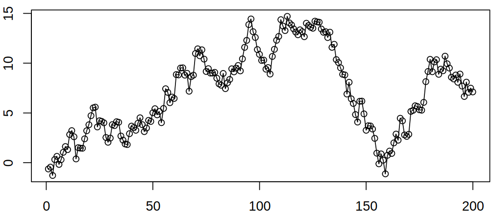
Random walk is a stochastic process that emerges from the cumulative sum of white noise. Let \(\rve_1, \rve_2, \dots\) be a sequence of independent, identically distributed random variables with mean \(0\) and variance \(\procVar\). Then define \[ \rnd X_t = \sum_{j = 1}^t \rve_j,\; t = 1,2, \dots \] or in other words \[ \rnd X_1 = \rve_1, \quad \rnd X_{t+1} = \rnd X_t + \rve_t, \; t = 2,3, \dots, \] where \(\rve_t\) are the steps taken by the “random walker”, \(\rnd X_t\) is his position at time \(t\).