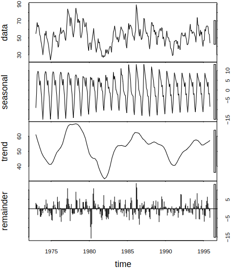
data(hsales, package="fma")
plot(decompose(hsales,type="additive"))6 Decomposition Techniques and Simple Prediction Methods
6.1 Decomposition
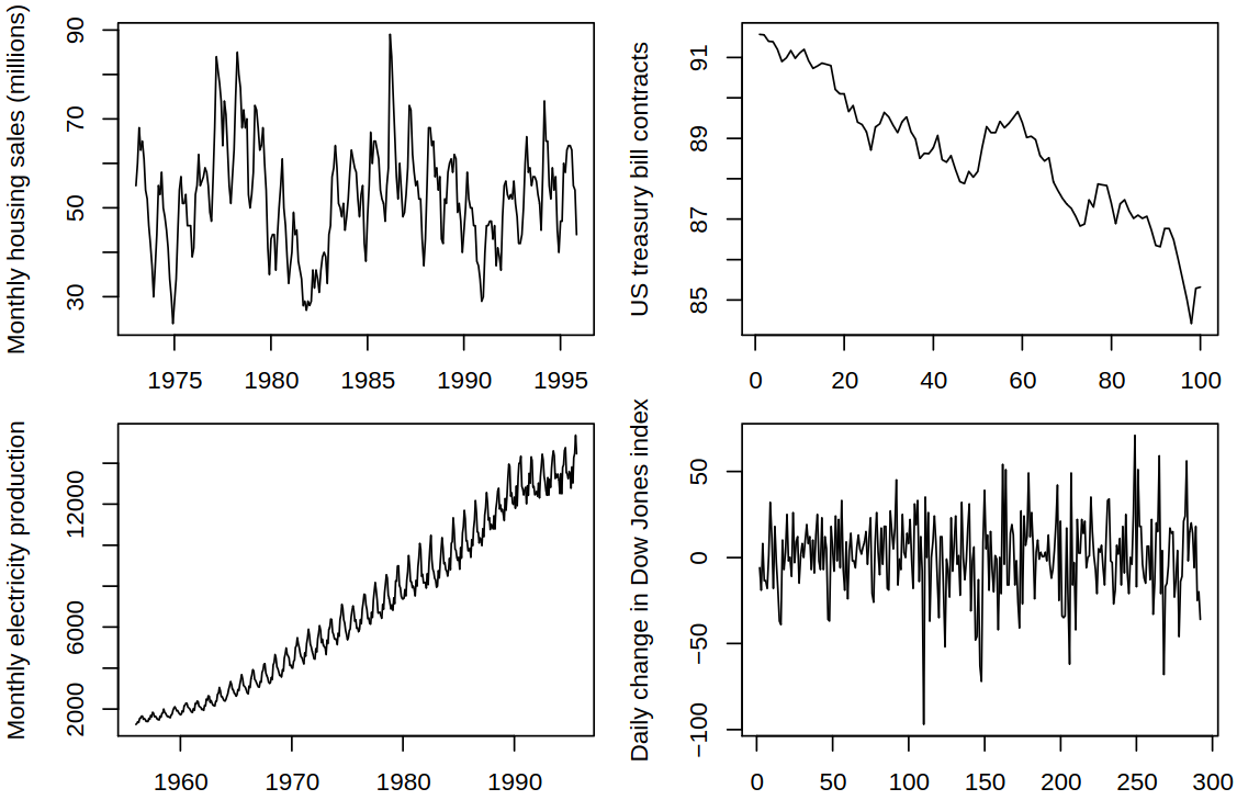
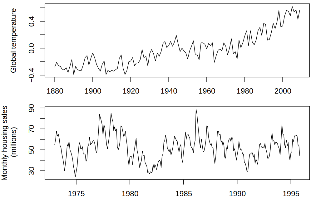
Consider a series with different components, see Figure 6.1 for examples.
As we did earlier, our goal will be to decompose \(\rnd X_t\) as \[ \rnd X_t = f(T_t, S_t, \rnd E_t) \] where
- \(T_t\) is the trend,
- \(S_t\) is the seasonal component (length of season \(s\), e.g. \(s = 12\)),
- \(\rnd E_t\) is the random component (remainder, irregular, error term).
All in all, our approach is similar to what we’ve used before, but now we allow the components to vary in a flexible, non-parametric way. As examples of this decomposition, consider
- Additive decomposition \[ \rnd X_t = T_t + S_t + \rnd E_t; \]
- Multiplicative decomposition \[ \rnd X_t = T_t S_t \rnd E_t. \]
In general, the goal of the decomposition is to aid us in exploratory analysis or it can serve as a preliminary step before the analysis of the random component.
6.1.1 Classical Decomposition
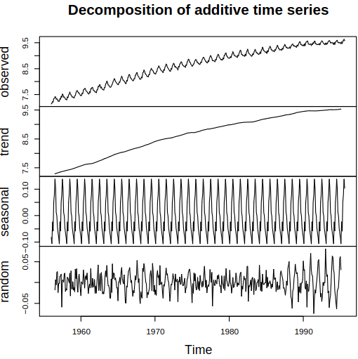
Consider a “classical” additive decomposition of \(\rnd X_t\) as \[ \rnd X_t = T_t + S_t + \rnd E_t, \] where \(T_t\) is allowed to change in time flexibly. Moreover, \(S_t\) is periodic with period \(s\) with the seasonal indices presumed to be constant in time. So our modeling procedure goes:
- estimate \(T_t\) by the moving average of order \(s\) to obtain \(\estim{\rnd T}_t\);
- calculate the de-trended \(\rnd X_t - \estim{\rnd T}_t\);
- estimate the seasonal component for each season (e.g. month) by averaging the de-trended values for that season. Then we adjust them so that they add up to zero, by which we produce \(\estim{\rnd S}_t\);
- calculate the remainder component \(\estim{\rnd E}_t = \rnd X_t - \estim{\rnd T}_t - \estim{\rnd S}_t\).
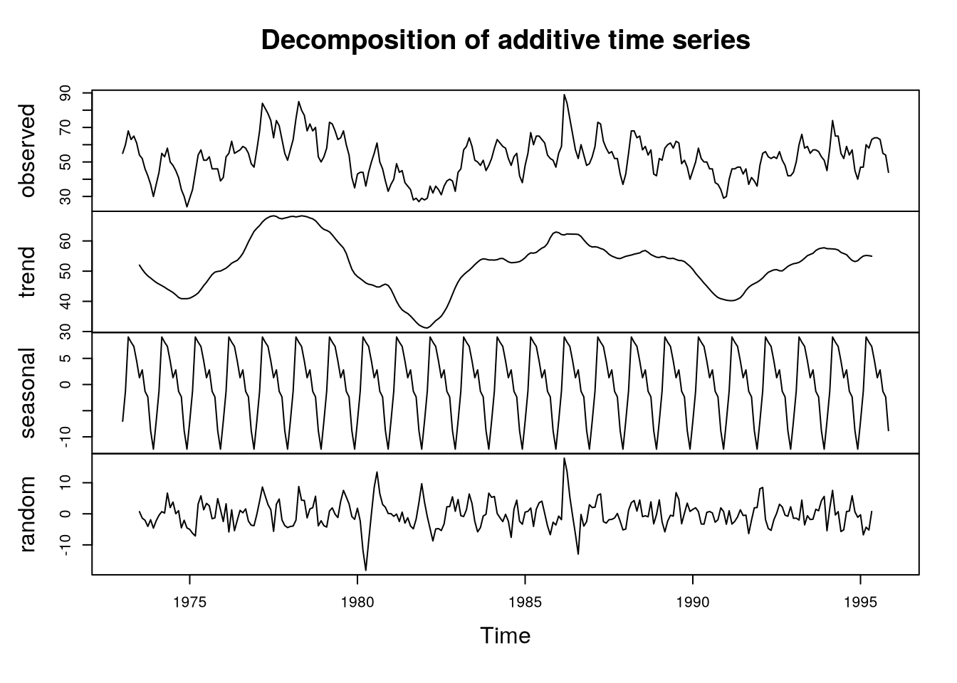
Example 6.1 As an example, consider housing sales and the following code:
6.1.2 Multiplicative Classical Decomposition
This time we decompose \(\rnd X_t\) as \[ \rnd X_t = T_t S_t \rnd E_t \] with the same interpretation of the used symbols. Our modeling process stays almost the same as well:
- estimate \(\rnd T_t\) by the moving average of order \(s\) to obtain \(\estim{\rnd T}_t\);
- calculate the de-trended \(\rnd X_t / \estim{\rnd T}_t\);
- estimate the seasonal component for each season (e.g. month) by averaging the de-trended values for that season. Then we adjust them so that they add up to zero, by which we produce \(\estim{\rnd S}_t\);
- calculate the remainder component \(\estim{ \rnd E}_t = \frac {\rnd X_t} {\estim{\rnd T}_t \estim{\rnd S}_t}\).
6.1.3 Problems with classical decomposition
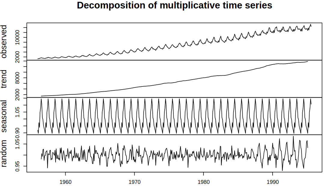
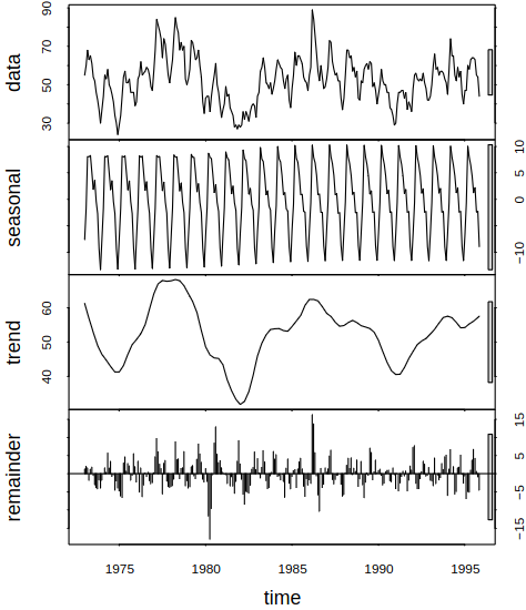
As we might have noticed, there are certain problems with the classical decomposition. For one, due to the moving average estimation, the trend is not available at the beginning and end of our data (roughly at the first and last \(s/2\) time points). Also, we assumed constant seasonal effects, which may be OK for some series but not for all, see Figure 6.2.
Basically, the latter problem boils down to the question of if the trend is allowed to vary flexibly for exploratory analysis, why not the seasonals?
6.1.4 STL Decomposition
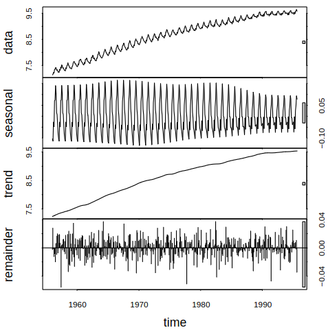
Once again, consider additive decomposition of \(\rnd X_t\) as \[ \rnd X_t = T_t + S_t + \rnd E_t, \] though this time we estimate \(T_t, S_t, \rnd E_t\) using STL (Seasonal and Trend decomposition using Loess). Hence now, \(T_t\) is allowed to change in time in a flexible way, and the smoothness of the trend component can be controlled. Also, \(S_t\) is now allowed to change in time flexibly (not only periodically), and the rate of change can also be controlled. Both time-varying functions are estimated nonparametrically by loess, which is a nonparametric regression technique similar to kernel smoothing.
STL decomposition is only additive, so one needs to use \(\log\) or Box-Cox (see Definition 5.1) transformations for different types of decompositions.
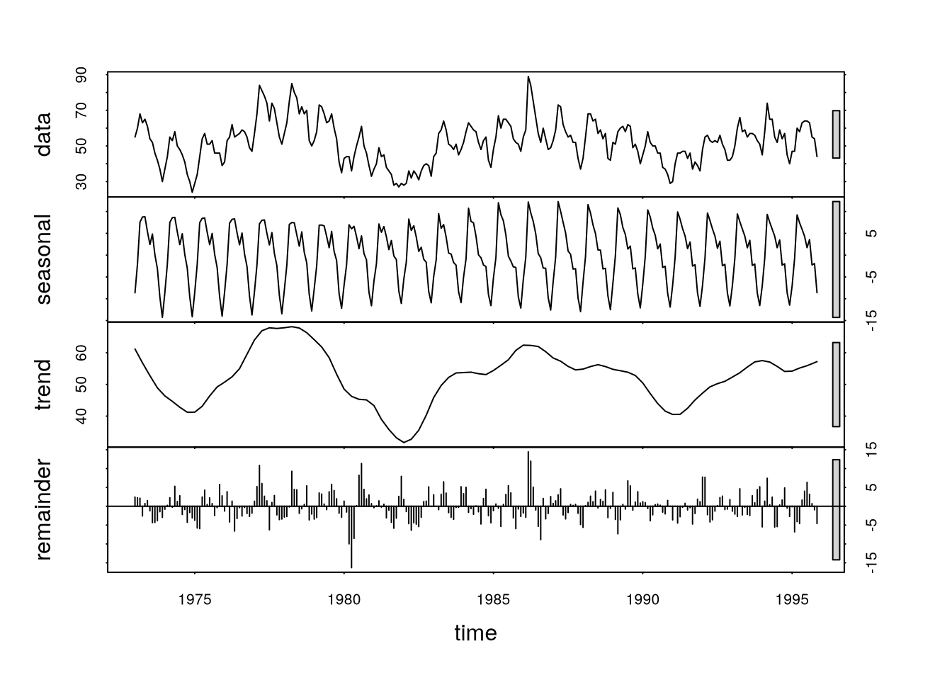
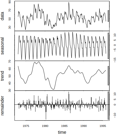
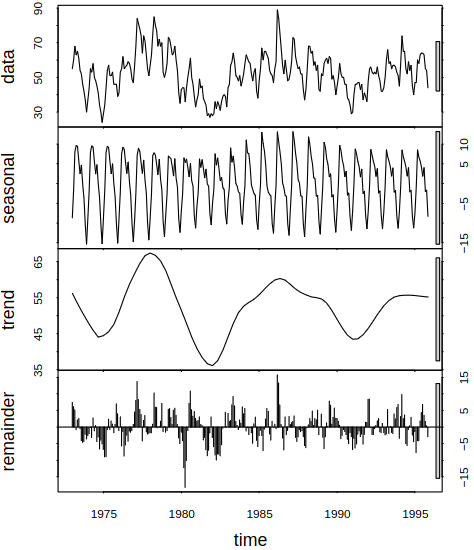
Recall the classical decomposition of housing sales, see Example 6.1. We now decompose the same data using STL with the following code:
In general, STL decomposition first estimates the trend by loess. Then it de-trends the series and applies loess smoothing to each seasonal sub-series. It follows by removing the seasonal component. All of these steps are iterated until a satisfying result is achieved (or another stopping condition is met).
6.1.5 Comparison of Classical and STL Decompositions
When comparing these two methods on the \(\log\)-transformed electricity data, see Example 6.2, we see that the classical decomposition fails to capture the decrease of seasonal effects at the end and as such, they propagate to the remainder component. What’s more, the remainder from STL looks far more random and irregular, compared to the one produced by the classical decomposition.
6.2 Exponential Smoothing
Let us now assume our goal is to predict (forecast) future values as a function of past observations. Therefore we need to incorporate changing the level, trend and seasonal patterns.
Let us presume we have observed data \(\rnd X_1, \dots, \rnd X_n\) and we want to predict the future values \(\rnd X_{n+h}\) for \(h = 1,2,\dots\). Firstly, let us introduce a new notation \(\predict{X}{n+h}{n}\) to denote the prediction of \(\rnd X_{n+h}\) from observed \(\rnd X_1, \dots, \rnd X_n\). Moreover, we assume there is no systematic trend or seasonal effects. This means that the level of the process can vary with time but we have no information about the likely direction of these changes.
As such, we model our data with \[ \rnd X_t = \mu_t + \rnd e_t, \] where \(\mu_t\) is the varying mean of the process and \(\rnd e_t\) are independent random inputs with mean \(0\) and standard deviation \(\sigma\). Also, let \(\rnd a_t\) be an estimate of \(\mu_t\).
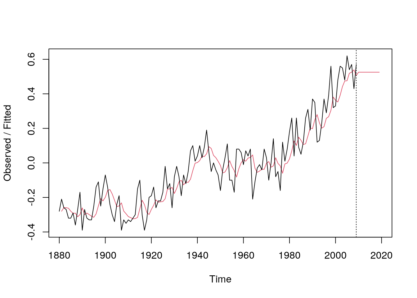
Since there is no systematic trend, \(\rnd X_{n+h}\) can be simply predicted by the forecating equation: \[ \predict{X}{n+h}{n} = \rnd a_n. \] The estimate \(\rnd a_t\) can be obtained using the same way – no systematic trend implies that it is reasonable to estimate \(\mu_t\) by a weighted average of our estimate at time \(t-1\) and the new observation at time \(t\), i.e. by the smoothing equation \[ \rnd a_t = \alpha \rnd X_t + (1 - \alpha) \rnd a_{t-1} \tag{6.1}\] for some \(\alpha \in (0,1)\). Here we call \(\alpha\) a smoothing parameter. For \(\alpha\) close to \(1\), we put more weight on the new observation \(\rnd X_t\), which produces fast changes. On the other hand, for \(\alpha\) close to \(0\), we put more weight on the previous estimate \(\rnd a_{t-1}\), which forces changes to be rather slow. We can repeat the process behind (6.1) with the back-substitution method to get \[ \rnd a_t = \alpha \rnd X_t + \alpha(1 - \alpha)\rnd X_{t-1} + \alpha (1 - \alpha)^2 \rnd X_{t-2} + \dots \]
From this arises the name exponential smoothing or exponentially weighted moving average.
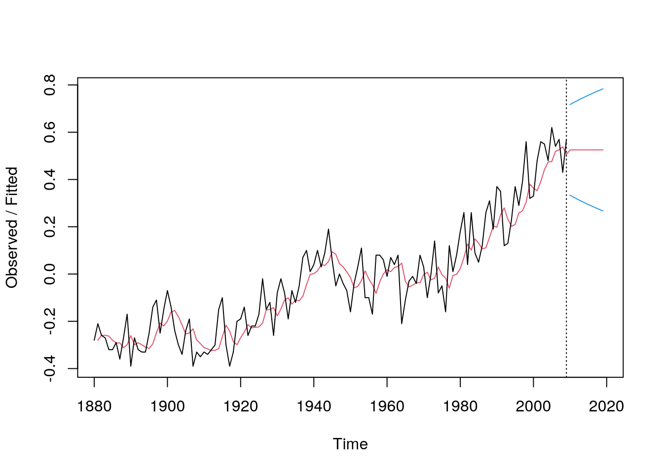
As an example, consider exponential smoothing applied to global temperatures with the following code
data(gtemp,package="astsa")
 # fit the model
m = HoltWinters(gtemp,
    alpha=.3,
    beta=F,
    gamma=F
)
# compute predictions 10 years ahead
p = predict(m,10)
plot(m,p,main="")6.2.1 Selection of the smoothing parameter
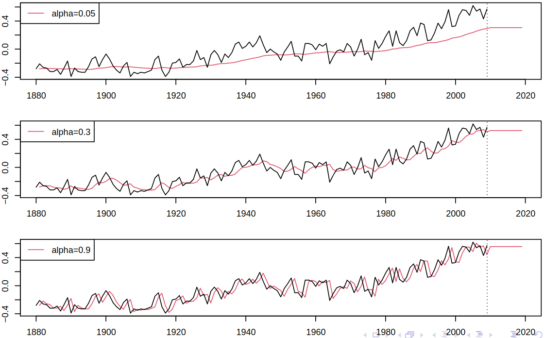
As always, the exact selection of the smoothing parameter is a tricky matter. In general, small \(\alpha\) leads to over-smoothing and the smoothed level lacks flexibility, while big \(\alpha\) promotes under-smoothing, and the smooth level follows the data too closely. As heuristics, values around \(0.2\) to \(0.3\) are often recommended.
In linear regression we estimate parameters by minimizing the sum of squared errors, so here we can use the same idea. Surely, we can estimate the unknown parameters and the initial values for exponential smoothing by minimizing the sum of squared errors. In this case, we consider the prediction errors \(\rnd X_t - \predict{X}{t}{t-1}\). Putting all of this together we get that the criterion to minimize is \[ \sum_{t = 1}^n \brackets{\rnd X_t - \predict{X}{t}{t-1}}^2. \]
Unlike with ordinary least squares, this problem is non-linear and numerical methods (like Newton’s method) must be used.
In R one can use HoltWinters to estimate the smoothing parameter \(\alpha\).
What’s more, we can construct prediction intervals that will contain the future observation \(\rnd X_{n+h}\) with a high probability, e.g. \(0.95\), as in Figure 6.7 using the following code.
6.3 Holt’s linear method
Exponential smoothing assumes no trend of the level, predictions are constant, but this may be insufficient, e.g., global temperatures exhibit temporary trends. As such, we use Holt’s method which incorporates trends. Therefore we predict \(\rnd X_{n+h}\) from data up to time \(n\) by \[ \predict{X}{n+h}{n} = \rnd a_n + h \rnd b_n, \] for \(h = 1,2,\dots\), where \(\rnd a_n\) is an estimate of level, and \(\rnd b_n\) is an estimate of slope. So now we estimate the level at \(t\) by a combination of the new observation and linearly extrapolated previous estimate \[ \rnd a_t = \alpha \rnd X_t + (1 - \alpha) (\rnd a_{t-1} + \rnd b_{t-1}). \] Similarly, we estimate the slope by a combination of the slope of the new level change and the previous estimate \[ \rnd b_t = \beta(\rnd a_t - \rnd a_{t-1}) + (1 - \beta) \rnd b_{t-1}. \] Same as before, \(\alpha, \beta \in (0,1)\) are smoothing parameters controlling the flexibility of the estimates \(\rnd a_t,\rnd b_t\) – how quickly they adapt to new data.
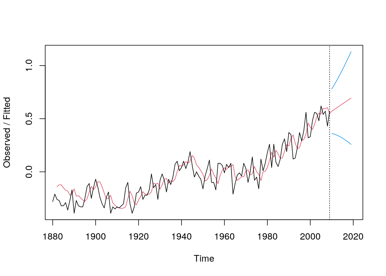
To demonstrate this method, consider the following code, which plots Figure 6.8.
# fit the model
m = HoltWinters(gtemp,
    alpha=.4,
    beta=.1,
    gamma=F
)
# point and interval predictions
p = predict(m,10,
    prediction.interval=TRUE
)
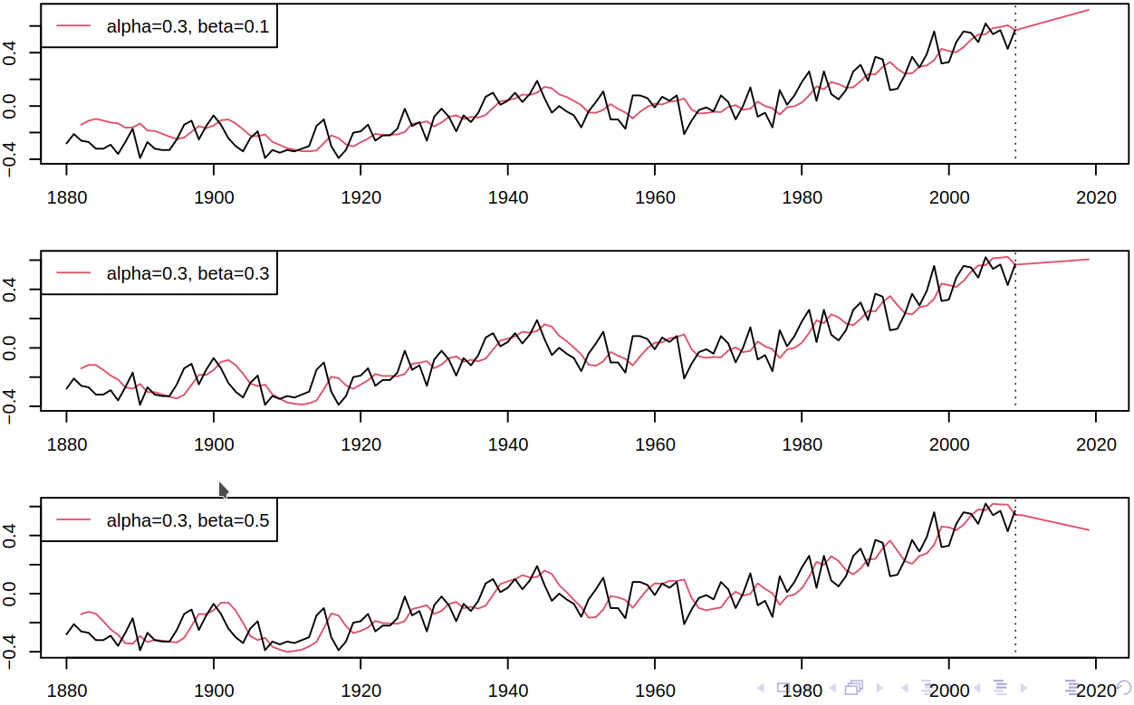
plot(m,p,main="")To get a better understanding of the effect of change of the smoothing parameters \(\alpha, \beta\), we may plot smoothed levels for a fixed \(\alpha\) and different \(\beta\) (we’ve seen the effect of \(\alpha\) already, see Figure 6.6).
Again, we can optimize for the value of parameters against some criterion using, for example, least squares.
6.4 Holt-Winters method
While Holt’s linear method is more general than pure exponential smoothing, it still lacks any seasonality. An extension of Holt’s linear method to include the aforementioned seasonality is called a Holt-Winters method. Consider a season with length \(p\), e.g. \(p = 12\). We now predict \(\rnd X_{n+h}\) from data up to time \(n\) by \[ \predict{X}{n+h}{n} = \rnd a_n + h\rnd b_n + \rnd s_{\periodPart n h p}, \] for \(h = 1,2,\dots\), where
- \(\rnd a_n\) is an estimate of the level;
- \(\rnd b_n\) is an estimate of the slope;
- \(\rnd s_{\periodPart n h p}\) is an estimate of the seasonal effect at time \(\periodPart n h p\) (i.e., the corresponding seasonal effect within the last p observation times, e.g., the seasonal of the last observed April if \(n + h\) is in April).
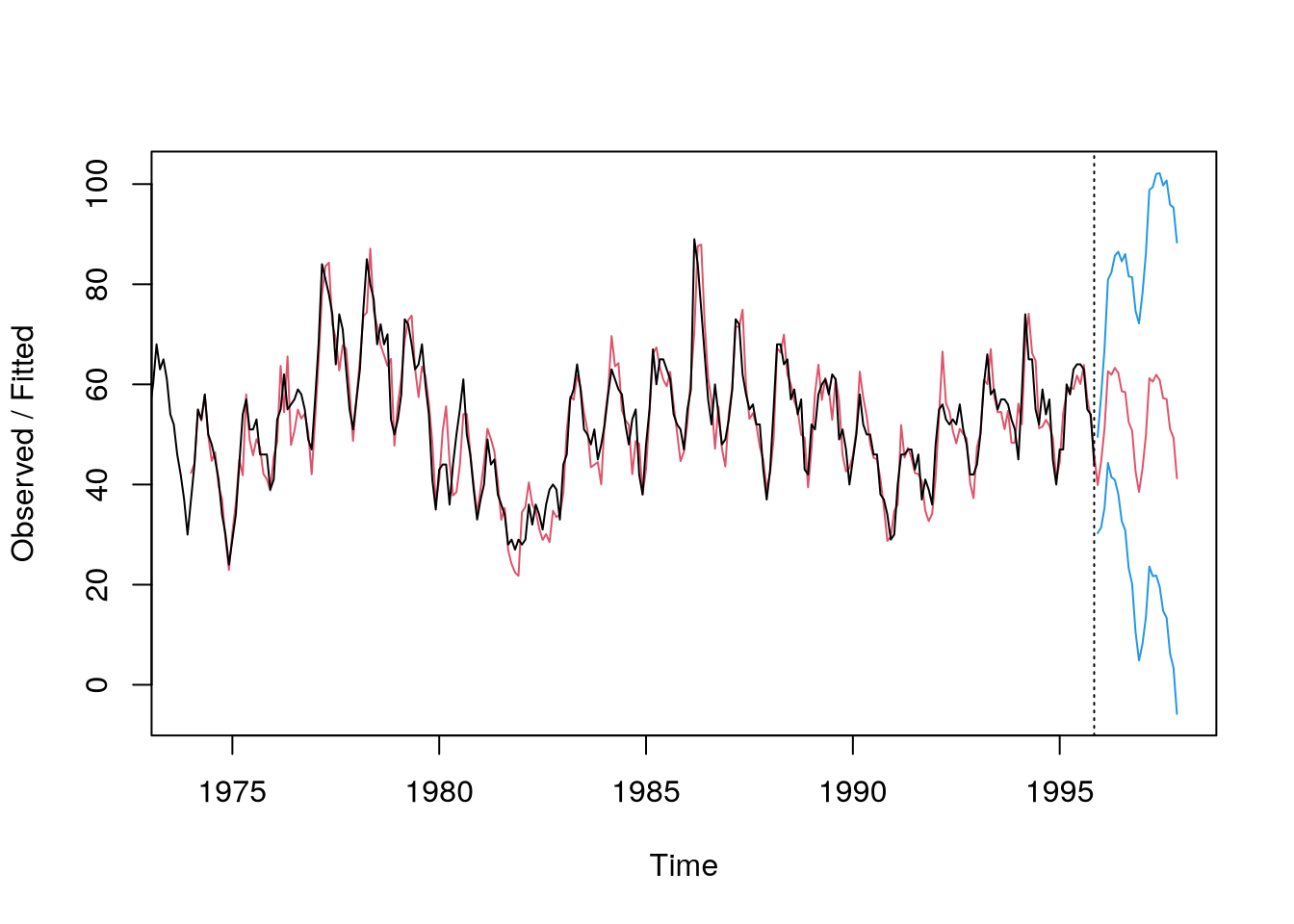
The updating equations now are \[ \begin{aligned} \rnd a_t &= \alpha (\rnd X_t - \rnd s_{t-p}) + (1 - \alpha) (\rnd a_{t-1} + \rnd b_{t-1}), \\ \rnd b_t &= \beta(\rnd a_t - \rnd a_{t-1}) + (1 - \beta)\rnd b_{t-1}, \\ \rnd s_t &= \gamma(\rnd X_t - \rnd a_t) + (1 - \gamma)\rnd s_{t-p}, \end{aligned} \] where \(\alpha, \beta, \gamma \in (0,1)\) are the smoothing parameters. Again, to demonstrate consider the housing sales data and the following code
