set.seed(1)
x = filter(rnorm(202),
    sides=1,
    filter=c(1,.6,.9),
    method="convolution"
)[-(1:2)]
acf(x,ci.type="ma",lag.max=20)4 Estimation of the autocorrelation function
There are multiple approaches when trying to determine the autocorrelation function \(\acf\) of given data. The first obvious way is to determine \(\acf\) from the used model. While this works, their autocorrelation \(\acf\) is often very complicated. It should be also said that direct modeling of the autocorrelation \(\acf\) is difficult. The second way is determining the form of acf \(\acf\) directly from data without any underlying model assumptions. These estimates can be used for inference on the relationships between the variables and for identifying a good model.
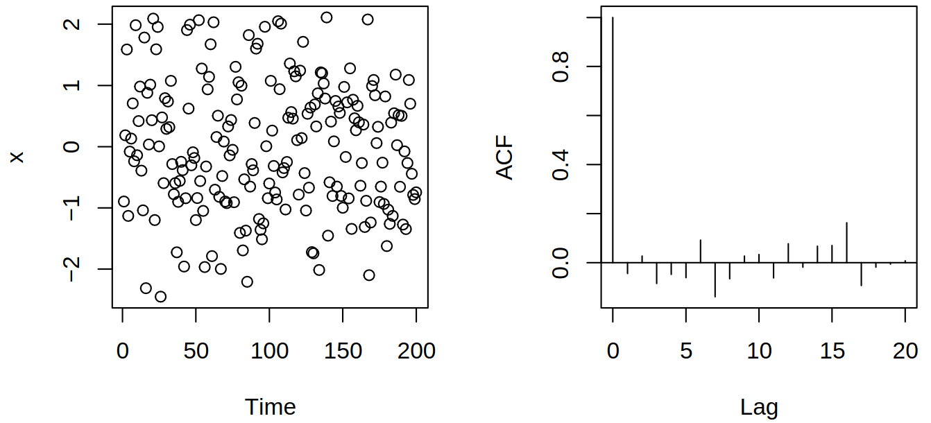
Therefore we are in a situation where we have observations \(\rnd X_1, \dots, \rnd X_n\) of a stationary series and let our goal be to estimate \[ \acov(h) = \cov(\rnd X_t, \rnd X_{t+h}) = \Expect{(\rnd X_t - \mu)(\rnd X_{t+h} - \mu)}. \] Naturally, we can use the empirical counterpart \[ \estim{\rnd \acov}(h) = \frac {\sum_{i = 1}^{n-h} (\rnd X_i - \Avg{\vr X})(\rnd X_{i+h} - \Avg{\vr X})} n, \] where alternatively the denominator can be \(n-h\) or something similar, but \(n\) is typically used in the context of time series (for positive semi-definiteness and simplification of acf \(\acf\)). Now we can estimate the autocorrelation function \(\acf(h) = \frac {\acov(h)} {\acov(0)}\) by \[ \estim{\rnd \acf}(h) = \frac {\estim{\rnd \acov}(h)} {\estim{\rnd \acov}(0)} = \frac {\sum_{i = 1}^{n-h} (\rnd X_i - \Avg{\vr X})(\rnd X_{i+h} - \Avg{\vr X})} {\sum_{i = 1}^n (\rnd X_i - \Avg{\vr X})^2}. \] We can picture this with simulated white noise and its correlogram (plot of the estimated autocorrelation function \(\acf\)), see Figure 4.1.
4.1 Properties of the empirical autocovariance and autocorrelation
Under the non-restrictive assumptions, \(\estim{\rnd \acov}(h)\) and \(\estim{\rnd \acf}(h)\) consistently estimate \(\acov(h), \acf(h)\) respectively. Furthermore, we would like to see whether the autocorrelations (bars in the correlogram) are important or not. Therefore we will study the asymptotic distribution of \[ \estim{\vr c}(h) = (\estim{\rnd \acov}(0), \estim{\rnd \acov}(1), \dots, \estim{\rnd \acov}(h))\Tr \] and \[ \estim{\vr r}(h) = (\estim{\rnd \acf}(1), \dots, \estim{\rnd \acf}(h))\Tr \] for \(n \to \infty\).
Theorem 4.1 If \(\set{\rnd X_t}\) is a stationary process, then, under certain assumptions, for any fixed \(h\) the vector of estimated autocovariances \(\estim{\vr c}(h)\) is approximately (for \(n \to \infty\)) normally distributed, i.e., \[ n^{1/2} (\estim {\vr c}(h) - \vi c(h)) \inDist \normalDist_{h+1}(0, \vi V), \] where \(\vi c(h) = (\acov(0), \dots, \acov(h))\Tr\).
Note that the matrix \(\vi V\) can be given explicitly. In particular, if the process consists of uncorrelated variables \((\acov(j) = 0, j \neq 0)\), then \(\vi V\) is diagonal with \(V_{jj} = \acov(0)^2\) for \(j > 0\) (hence the components of \(\estim{\vr c}(h)\) are asymptotically independent). Examples of certain conditions are again given in the slides, but one can remember that ARMA processes satisfy them
4.2 Asymptotic qualities of the sample autocorrelation
Most often, we wish to make inferences about the dependence structure regardless of scale and we would like to have the asymptotic distribution for autocorrelations rather than autocovariances. The sample autocovariances are (more or less) sums of variables (some central limit theorem is behind the proof). The sample autocorrelation \[ \estim{\rnd \rho}(j) = \frac {\estim{\rnd \acov}(j)} {\estim{\rnd \acov}(0)} \]
is a non-linear function (ratio) of the autocovariances. So the question is: Can we deduce the asymptotic distribution of a function of an estimator if we have it for the estimator itself?
4.3 Limit theorems
Theorem 4.2 (Continuous mapping) Let \(g\) be a continuous function. Then
- if \(\rnd R_n \inProbWhen{n \to \infty} \rnd R\), then \(g(\rnd R_n) \inProbWhen{n \to \infty} g(\rnd R)\)
- or if \(\rnd R_n \inDistWhen{n \to \infty} \rnd R\), then \(g(\rnd R_n) \inDistWhen{n \to \infty} g(\rnd R)\),
where the \(g\) actually needs to only be continuous on a set \(X\) such that \(P(\rnd R \in X) = 1\).
Clearly, we can use the continuous mapping Theorem 4.2 when we have a random variable \(\estim{\rnd v}_n\), which consistently estimates a variance of interest. Then \(\estim{\rnd v}_n^{1/2}\) consistently estimates the corresponding standard deviation.
Theorem 4.3 (Slutsky’s) Let \(\rnd R_n \inDistWhen{n \to \infty} \rnd R\) and \(\rnd S_n \inProbWhen{n \to \infty} s\), where \(s\) is a non-random constant. Then \[ \rnd R_n \rnd S_n \inDistWhen{n \to \infty} s \rnd R \quad \& \quad \rnd R_n + \rnd S_n \inDistWhen{n \to \infty} \rnd R + s. \]
Again, a familiar use of Slutsky’s Theorem 4.3 might be if we have \[ n^{1/2} (\estim{\rtht}_n - \tht) \inDistWhen{n \to \infty} \normalD{0,v}, \qquad \estim{\rnd v}_n \inProbWhen{n \to \infty} v, \] then \[ \estim{\rnd v}_n^{-1/2}n^{1/2}(\estim{\rtht}_n - \tht) \inDistWhen{n \to \infty} \normalD{0,1}. \]
4.4 Delta method
Let \(\estim{\vrr \theta}_n \in \R^p\) be a random vector and assume it is asymptotically normal with mean \(\vi \theta\) and variance matrix \(a_n^{-2}\vi V\), i.e. \[ a_n(\estim{\vrr \theta}_n - \vi \theta) \inDistWhen{n \to \infty} \normalDist_p\brackets{\vi 0,\vi V}. \]
Our goal is now to find the asymptotic distribution of \(\vi g(\estim{\vrr \theta}_n)\), where \(\vi g: \R^p \to \R^q\). If \(\vi g\) is continuously differentiable at \(\vi \theta\) with \(\jacobi \vi g(\vi \theta) = \partialOp{\vi \theta} \vi g(\vi \theta) \in \R^{p\times q}\), then by Taylor series, Theorem 4.2 and Theorem 4.3, we get
\[ a_n \brackets{\vi g(\estim{\vrr \theta}_n) - \vi g(\vi \theta)} = \jacobi \vi g(\vi \theta^*) a_n(\estim{\vrr \theta}_n - \vi \theta) \onBottom{\onTop{\to}{d}}{n \to \infty}\\ \jacobi \vi g(\vi \theta) \normalDist_p(\vi 0,\vi V) = \normalDist_q\brackets{\vi 0, \jacobi \vi g(\vi \theta) \cdot \vi V \cdot \jacobi \vi g(\vi \theta)\Tr}. \]
Here the “delta” stands for differentiation.
The delta method is a very useful general tool (bear in mind it is not limited to this particular context).
4.5 Asymptotic qualities of the sample autocorrelation – cont.
Consider \(\vi g(x_0, \dots, x_h) = (x_1/x_0, \dots, x_h/x_0)\Tr\), then \[ \estim{\vr \acf}(h) = \vi g(\estim{\vr c}(h)), \quad \vi \acf(h) = \vi g(\vi c(h)), \] and also \(\vi g\) has the \(h \times (h+1)\) Jacobi matrix of partial derivatives in form \[ \jacobi \vi g(x_0, \dots, x_h) = \frac 1 {x_0^2} \mtr{ -x_1 & x_0 & 0 & \cdots & 0 \\ -x_2 & 0 & x_0 & \cdots & 0 \\ \vdots & \vdots & \vdots & \ddots & \vdots \\ -x_h & 0 & 0 & \cdots & x_0 }. \]
At \(\vi x = \vi c(h)\), this is \(\jacobi \vi g(\vi c(h)) = \frac 1 {\acov(0)} \mtr{-\vi r(h) & \ident_h}\) with \(\ident_h\) denoting \(h\times h\) identity matrix. Then \(\estim{\vr r}(h)\) is approximately normal with mean \(\vi r(h)\) and covariance matrix \(n^{-1} \jacobi \vi g(\vi c(h)) \vi V \jacobi \vi g(\vi c(h))\Tr\).
Theorem 4.4 If \(\set{\rnd X_t}\) is a stationary process, then, under certain assumptions, for any fixed \(h\) the vector of estimated autocorrelations \(\estim{\vr r}(h)\) is approximately (for \(n \to \infty\)) normally distributed, i.e.
\[
n^{1/2}(\estim{\vr r}(h) - \vi r(h)) \inDist \normalDist_h(\vi 0,\vi W),
\] where \(\vi W\) is the \(h \times h\) matrix with entries given by the Barlett formula \[
W_{ij} = \sum_{k = 1}^\infty \brackets{
\acf(k+i) + \acf(k - i) + 2\acf(i) \acf(k)
} \cdot \brackets{
\acf(k+j) + \acf(k - j) + 2\acf(j) \acf(k)
}.
\]
For white noise (that is, \(\acf(t) = 0, t \neq 0\)) we get \(W_{ij} = 1\) for \(i = j\), \(W_{ij} = 0\) otherwise.
4.5.1 Sample autocorrelation of white noise
Theorem 4.5 If \(\set{\rnd X_t}\) is a sequence of iid random variables, then, under certain assumptions, for any \(h\) the vector of estimated autocorrelations \(\estim{\vr r}(h)\) is approximately (for \(n \to \infty\)) normally distributed with mean zero, variances \(1/n\) and independent components, i.e. \[ n^{1/2}\estim{\vr r}(h) \inDistWhen{n \to \infty} \normalDist_h(0, \ident_h). \]
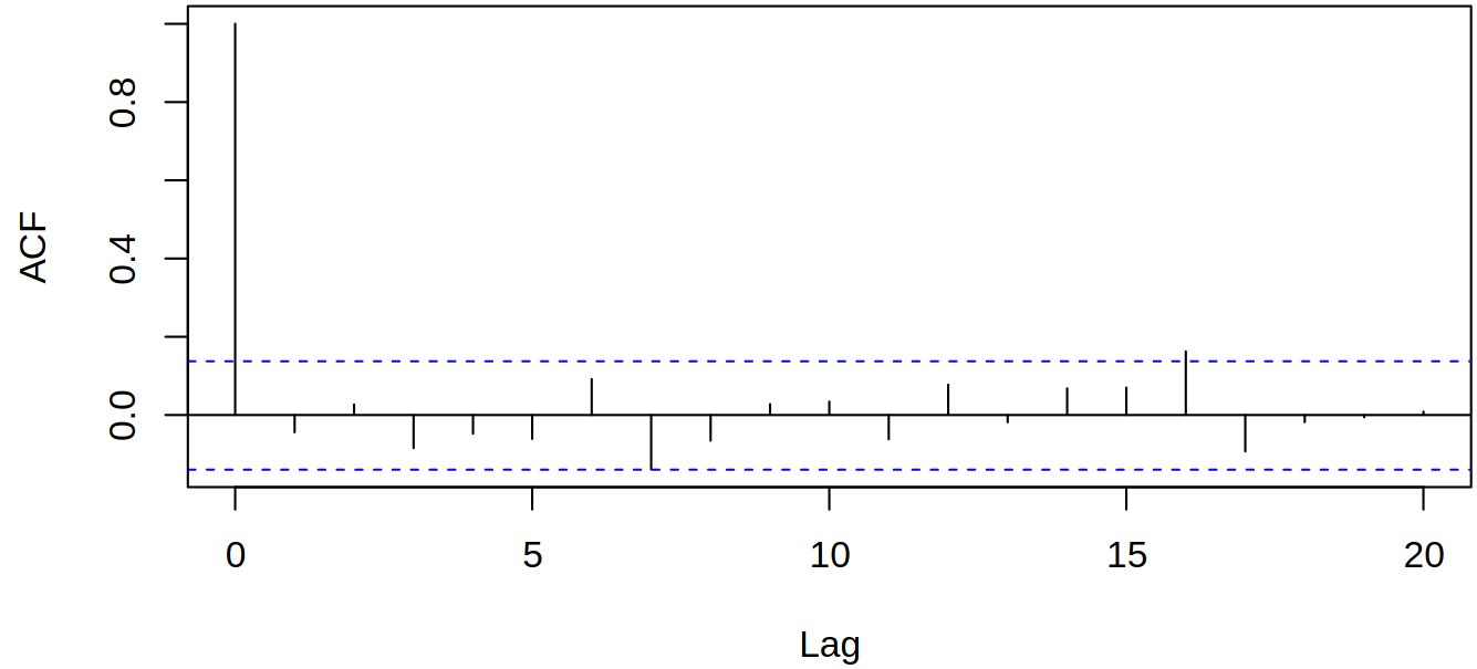
It should be clear that Theorem 4.5 follows from Theorem 4.4. This allows us to test certain hypotheses because \(\estim{\rnd \acf}(j) \dot{\sim} \normalD{0, 1/n}\) under independence. Hence \(\estim{\rnd \acf}(j)\) should be between \(−1.96/\sqrt n\) and \(1.96/\sqrt n\) with approximate probability 95 % under independence
4.6 Inference about the autocorrelation structure
Here in Figure 4.2, the limits are at \(\pm 1.96/\sqrt n\). At lag \(j\), they indicate the rejection regions for testing the null hypothesis of no autocorrelation against the alternative that \(\acf(j) \neq 0\). When the estimated acf is between the blue dotted lines, i.e. in the confined region, we do not reject the null hypothesis. Due to the approximate independence, one can expect \(\alpha \times 100\%\) false rejections on average (e.g., 1 out of 20).
Although R calls it confidence intervals, it is more correctly a region of rejection/validity of sorts.
4.6.1 Asymptotic distribution of estimated acf of a moving average process
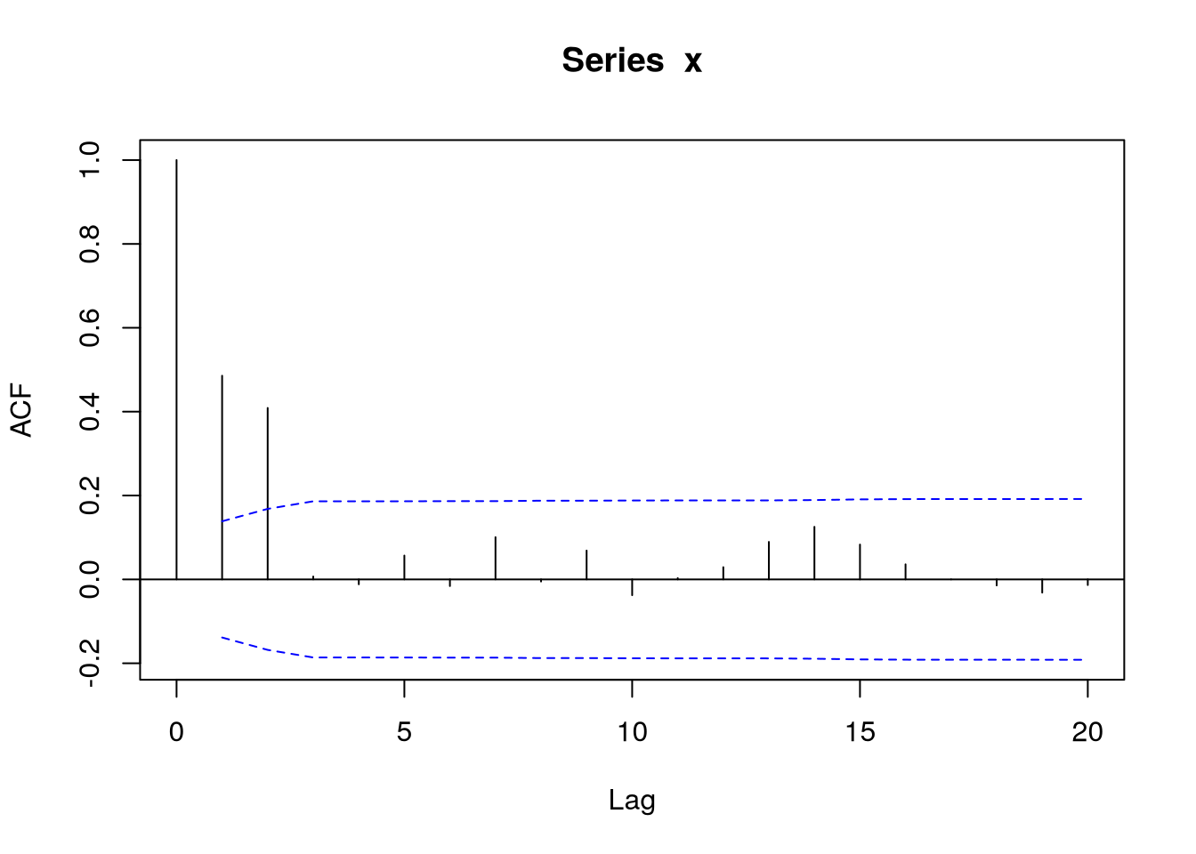
Consider white noise \(\set{\rve_t}\) and define \[ \rnd X_t = \rve_t + \theta_1 \rve_{t-1} + \dots + \theta_q \rve_{t-q}, \] for which we have already shown that \(\acf(j) = 0\) for \(j > q\). Thus we can test \[ \nullHypo: \acf(j) = 0, \; j \geq q+1 \quad \text{vs} \quad \altHypo: \acf(q+1) \neq 0, \; j \geq q + 2 \] and such we will reject \(\estim{\rnd \acf}(q+1)\) outside the limits \(\pm 1.96n^{-1/2}(1 + 2\sum_{k = 1}^q\estim{\rnd \acf}(k)^2)^{1/2}\). Note that there are wider limits because we put no restrictions on \(\acf(j), j \leq q\).
Example 4.1 Given a specific example \[ \rnd X_t = \rve_t + 0.6 \rve_{t-1} + 0.9\rve_{t-2}, \] we get, with the following code, these results:
4.6.2 The Ljung-Box test
Let us assume our goal is to test the global hypothesis of no autocorrelation. Begin with a null hypothesis \(\nullHypo: \acf(h) = 0\) for all \(h = 1,2,\dots, L\) for \(L \in \N\) and alternative \(\altHypo: \exists h \in \set{1, \dots, L}\), such that \(\acf(h) \neq 0\). We use the Box-Pierce test statistic \[ \rnd Q = n(\estim{\rnd \acf}(1)^2 + \dots + \estim{\rnd \acf}(L)^2). \] Now under \(\nullHypo\), \(\rnd Q\) is approximately \(\chi_L^2\) distributed – as such we will reject \(\nullHypo\) for \(\rnd Q > q_L(1-\alpha)\) where \(q_L(1 - \alpha)\) is \((1 - \alpha)\)-quantile of \(\chi_L^2\). In truth, the Ljung-Box test statistic reads (more precise for smaller values) \[ \rnd Q_* = n(n+2)\brackets{\frac{\estim{\rnd \acf}(1)^2}{n-1} + \dots + \frac{\estim{\rnd \acf}(L)^2}{n-L}}, \] which has the same approximate distribution (\(\rnd Q_*\) is much closer to chi-square than \(\rnd Q\))
Example 4.2 Consider the example (as an illustration) where the maximum delay of \(10\) was used:
We can’t choose too big a lag, because we would have too many parameters. As a heuristics, lag should be approximately \(< \frac n {10}\)
4.6.3 Maximum correlation test
We shall now aim to test whether any \(\acf\) at lags up to \(L\) is significant. We might have an idea to use single tests and combine them in \[ \rnd T = \max \brackets{\absval{\estim{\rnd \acf}(1)}, \dots, \absval{\estim{\rnd \acf}(L)}}. \] We can then look for \(c\) such that \(P(\rnd T > c) \onTop{=}{\cdot} \alpha\) under \(\nullHypo\) and as such, \(\estim{\rnd \acf}(1), \dots, \estim{\rnd \acf}(L)\) are approximately iid under \(\nullHypo\). Thus, also under \(\nullHypo\), \[ \begin{aligned} 1 - \alpha \onTop{=}{\cdot} P(\rnd T \leq c) &= P\brackets{\max \brackets{\absval{\estim{\rnd \acf}(1)}, \dots, \absval{\estim{\rnd \acf}(L)}} \leq c} \\ &= \prod_{j = 1}^L P\brackets{\absval{\estim{\rnd \acf}(j)} \leq c}\\ &= \prod_{j = 1}^L \brackets{ \Phi(n^{1/2}c) - \Phi(-n^{1/2}c) } \\ &= \brackets{2 \Phi(n^{1/2}c) - 1}^L. \end{aligned} \]
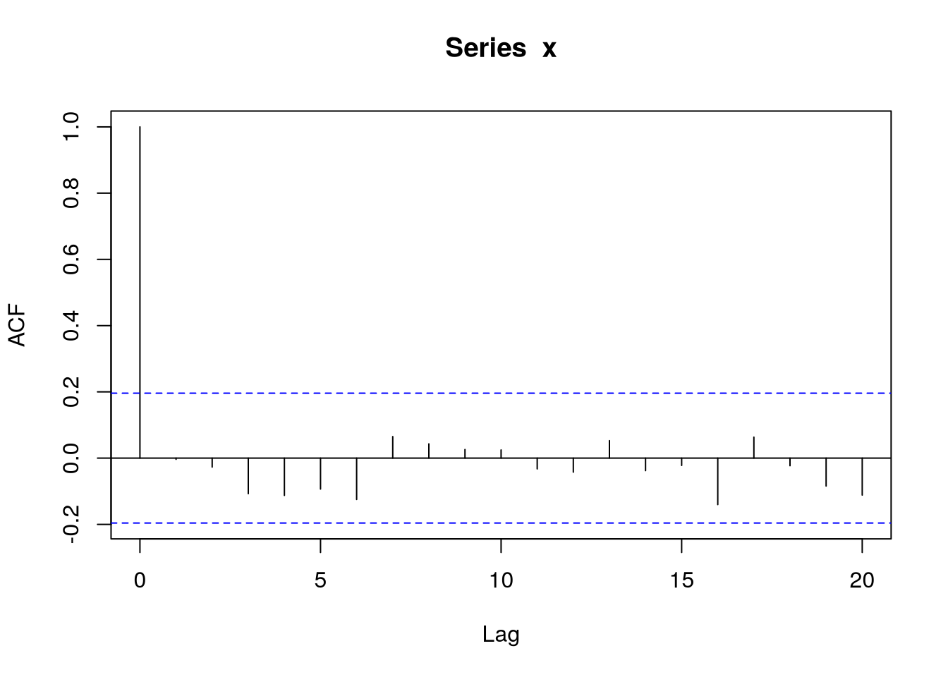
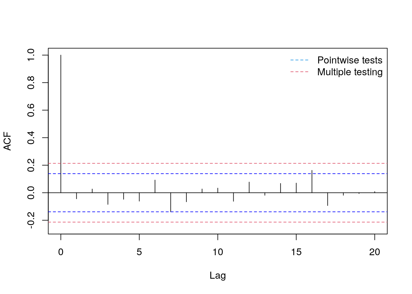
Hence the critical value is \(c = n^{-1/2} \Phi^{-1} \brackets{(1-\alpha)^{1/L}}\). Regions for testing multiple autocorrelations at once have boundaries at \(\pm c\) (whereas usual rejection regions in the correlogram are for tests about single autocorrelations).
set.seed(2); n = 200; x = rnorm(n); L = 20
# standard rejection limit for single tests
qnorm(.975)/sqrt(n)
[1] 0.1385904# rejection regions corrected for multiple testing
(max.lim = qnorm(.975^(1/L))/sqrt(n))[1] 0.2135257acf(x,
lag.max=L,
main="",
ylim=c(-.25,1)
)
abline(h=c(-1,1)*max.lim,
col=2,
lty=2
)
legend("topright",
legend=c("Pointwise tests","Multiple testing"),
col=c(4,2),
lty=2,
bty="n"
)4.6.4 Problems with acf estimation
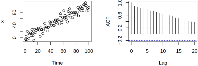
Surely, the \(\acf\) estimation and the correlogram make sense for stationary data. Now consider iid white noise \(\set{\rve_t}\) and define \(\rnd X_t = t + \rve_t\). Then \(\rnd X_t\) are independent variables, hence uncorrelated. If we directly apply the correlogram, we get misleading results, see Figure 4.3.
As this example shows, trends/deterministic components should be accounted for: e.g., model them by regression. Now consider the random walk \(\rnd X_t = \sum_{j = 1}^t \rve_j\) (this time series is non-stationary). Directly applying the correlogram to \(\rnd X_t\) indicates a complicated autocorrelation structure, see Figure 4.4.
On the other hand, applying the correlogram to the differentiated series \(\set{\rnd X_t - \rnd X_{t-1}}\) suggests a much simpler structure, see Figure 4.5.
Therefore transient trends should be accounted for, e.g., by differencing.
