3 Autocorrelation and stationarity
These notes are just a summary of the presentation given to us. As such, it is hard to comment on the true intent or intuition behind some of the presented results or sentences.
Thank you for your understanding.
As a starter, it is good to realize, that while correlation is useful, one should be mindful of what it really means.
3.1 Properties of autocovariance
As we’ve seen earlier in the Definition 2.2, the autocovariance function is defined as \[ \acov(s,t) = \cov(\rnd X_s, \rnd X_t), \quad s,t \in T \subset \R. \]
We may notice that for any \(k \in \N\), \(t_1, \dots, t_k \in T\), \(c_1, \dots, c_k \in \R\) \[ 0 \leq \Variance{\sum_{j = 1}^k c_j \rnd X_{t_j}} = \sum_{j = 1}^k \sum_{l = 1}^k c_j c_l \acov(t_j, t_l). \]
Hence the autocovariance function of a process with finite second moments is non-negative definite. The converse holds true as well – for any non-negative definite function \(g\) on \(T \times T\) there exists a stochastic process such that \(g\) is its autocovariance function. Because one can take matrices of the form \[ \vi V_{t_1, \dots, t_k} = \brackets{g(t_j, t_l)}_{j,l = 1}^k \] and consider the multivariate Gaussian distributions \(\normalDist_k\brackets{0, \vi V_{t_1, \dots, t_k}}\), then by the Daniell-Kolmogorov Theorem 2.1 there exists a Gaussian process with these finite-dimensional distributions.
3.2 Stationarity
Stationarity is a concept best introduced by illustrations.
Definition 3.1 (Strict stationarity) A process \(\set{\rnd X_t : t \in \Z}\) is said to be strictly stationary if the joint distribution of \(\rnd X_{t_1}, \dots, \rnd X_{t_k}\) is the same as the joint distribution of \(\rnd X_{t_1 + h}, \dots, \rnd X_{t_k + h}\) for all \(k \in \N, t_1, \dots, t_k \in \Z, h \in Z\), that is \[ F_{t_1, \dots, t_k}(x_1, \dots, x_k) = F_{t_1 + h, \dots, t_k + h}(x_1, \dots, x_k). \]
Definition 3.2 (Weak stationarity) A process \(\set{\rnd X_t : t \in \Z}\) is said to be weakly (weak-sense, second-order) stationary if the \(\mu_t\) is constant in time and \(\acov(s,t)\) depends only on the difference \(s-t\).
Any strictly stationary defined in Definition 3.1 process that has a finite mean and a covariance is also stationary in the weak sense. Also, if all joint distributions are Gaussian, then weak and strong stationarity are equivalent.
By convention, by simply “stationarity” we mean weak-sense stationarity – Definition 3.2.
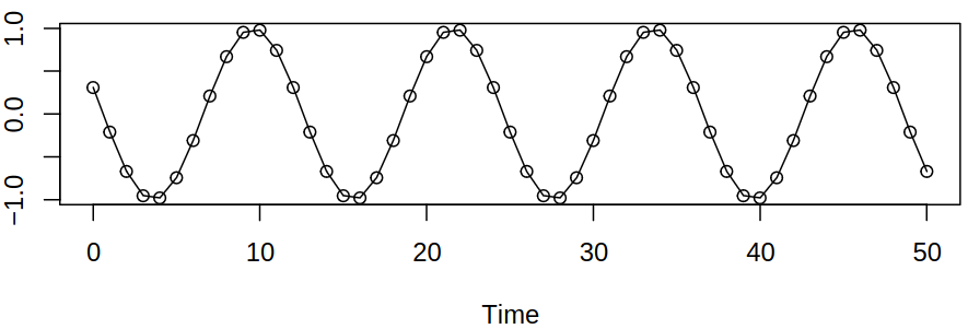
Example 3.1 Let us define \[ \rnd X_t = a \cos \brackets{2\pi (ft + \Phi)}, \quad t \in \Z, \tag{3.1}\] where \(a\) is the amplitude, \(f\) frequency (e.g. \(f = 1/12\)) and \(\Phi \in [0,1]\) is the phase. Consider now a random phase given by \(\Phi \sim \uniform ([0,1])\). It can be easily computed that \[ \expect \rnd X_t = \int_0^1 a \cos \brackets{2\pi (ft + \Phi)} \d\phi = 0. \]
From the Definition 2.2 and (3.1), it can be shown the autocovariance function \(\acov\) of this process has the form \[ \begin{aligned} \acov(s,t) &= \int_0^1 a \cos \brackets{2\pi (fs + \Phi)} a \cos \brackets{2\pi (ft + \Phi)} \d\Phi \\ &= \frac {a^2} 2 \cos \brackets{2 \pi (s-t)} \end{aligned} \tag{3.2}\] and as such, the autocorrelation is \(\acf(h) = \cos (2\pi fh)\), \(h \in \Z\). Hence this stationary process fulfills the criteria for WSS, see Definition 3.2.
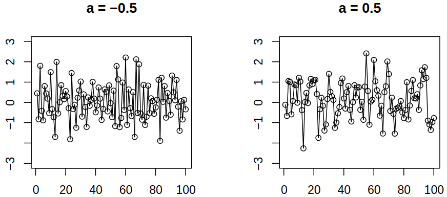
It should be noted that stationarity is the property of the distribution, not of the realization. Therefore one trajectory may not look stationary, but the process as a whole may be stationary, see Figure 3.1. In this example, it is precisely the random phase \(\Phi\), that makes the process stationary – independent random amplitude and phase would not be stationary.
Stationarity implies that properties of a given process are stable (aka do not change) in time. So with more and more data, we collect more and more information about the same, invariant structure. As such, averaging makes sense – without the stationarity averaging wouldn’t be meaningful, unless we know how the properties like the mean and the autocovariance function evolve in time.
Let now \(\set{\rnd X_t : t \in \Z}\) be a stationary time series. Let us assume we want to estimate the mean \(\mu = \expect \rnd X_t\), autocovariance function \(\acov(h) = \cov(\rnd X_t, \rnd X_{t+h})\) and autocorrelation function \(\acf(h) = \corr(\rnd X_t, \rnd X_{t+h})\) given the observed data \(\rnd X_1, \dots, \rnd X_n\). Therefore our goals are to find estimators \(\estim{\rnd \mu}, \estim{\rnd \acov}(h), \estim{\rnd \acf}(h)\), understand their properties and use them in statistical inference and graphics.
3.2.1 Estimation of the mean
As was stated before, we assume that \(\expect \rnd X_t = \mu\) for all \(t\). An obvious choice of the estimator would be the sample mean \[ \estim{\rnd \mu} = \Avg{\vr X} = \frac 1 n \sum_{i = 1}^n \rnd X_i. \] Its expected value is given by \[ \expect{\estim{\rnd \mu}} = \Expect{\frac 1 n \sum_{i = 1}^n \rnd X_i} = \mu, \] so \(\estim{\rnd \mu}\) is unbiased (regardless of the covariance structure of the process). To judge the quality of the estimator, let us look at its variance (see (3.2) for reference for derivation) \[ \begin{aligned} \variance \estim{\rnd \mu} &= \Variance{\frac 1 n \sum_{i = 1}^n \rnd X_i} \\ &= \frac 1 {n^2} \sum_{i = 1}^n \sum_{j = 1}^n \cov (\rnd X_i, \rnd X_j) \\ &= \frac 1 {n^2} \sum_{i = 1}^n \sum_{j = 1}^n \acov(i-j) \\ &= \frac 1 {n^2} \brackets{n \acov(0) + 2(n-1) \acov(1) + 2(n-2)\acov(2) + \dots + 2 \acov(n-1)} \\ &= \frac {\acov(0)} n \brackets{1 + 2 \sum_{i = 1}^{n-1} \frac {n-i} n \acf(i)}. \end{aligned} \tag{3.3}\]
When we perform estimation given by (3.3) on white noise, where \(\acf(h) = 0\) for \(h \neq 0\), we get \(\variance \estim{\rnd \mu} = \frac {\acov(0)} n\), so it follows the term \(2 \sum_{i = 1}^{n-1} \frac {n-i} n \acf(i)\) is a correction reflecting the impact of autocorrelation.
Example 3.2 Let \(a\) be a parameter, consider \(\set{\rve_t} \sim \WN{0}{\sigma^2/(1+a^2)}\) and define \[ \rnd X_t = \rve_t + a \rve_{t-1}. \]
We can compute \(\acov(0) = \sigma^2\), \(\acov(1) = a\sigma^2/(1+a^2)\) and \(\acov(h) = 0\) for \(\absval{h} > 1\), thus \(\acf(1) = a / (1 + a^2)\) and \(\acf(h) = 0\) for \(\absval{h} > 1\). Therefore this process has the same variance for all \(a\) but the correlation depends on \(a\).
When we now use the (3.3) to compute \(\variance \estim{\rnd \mu}\), we get \[ \variance \estim{\rnd \mu} = \frac {\sigma^2} n \brackets{1 + 2 \frac {n-1} n \frac a {1 + a^2}} \approx \frac {\sigma^2} n \brackets{1 + 2 \frac a {1 + a^2}} \] for very large \(n\). Thus \(\variance \estim{\rnd \mu} \to 0\) as \(n \to \infty\) – we can read this as meaning the more data we have, the better. For example
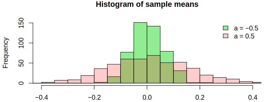
- for \(a = -0.5\), \(\variance \estim{\rnd \mu} \approx 0.2 \sigma^2/n\),
- for \(a = 0.5\), \(\variance \estim{\rnd \mu} \approx 1.8 \sigma^2/n\).
We can make the observation, that negative correlation improves the estimation of \(\mu\) – there will be more oscillations back and forth across the mean. On the other hand, a positive correlation reduces the accuracy of the estimate. Just as an illustration, we can simulate \(500\) realizations of length \(n = 100\) with \(\mu = 0\) and compute \(\estim{\rnd \mu}\) for each of them
In the slides, there are two more examples:
3.2.2 Consistency of the sample mean
We may recall the consistency of an estimator from previous courses.
Definition 3.3 (Consistency of an estimator) If \(\estim{\rtht}_n\) is an estimator of some parameter \(\tht\) from observations \(\rnd X_1, \dots, \rnd X_n\), it is called consistent when \(\estim{\rtht}_n \to \tht\) in some appropriate way, as \(n \to \infty\), for all values of \(\tht\).
The possible ways of convergence are:
- Almost surely \(\estim{\rtht}_n \convergeAS \tht \;\): \(\estim{\rtht}_n(\omega) \to \tht\) for all \(\omega \in A, P(A) = 1\) (strong consistency)
- In mean square \(\estim{\rtht}_n \inMeanSq \tht \;\): \(\Expect{(\estim{\rtht}_n - \tht)^2} \to 0\) (for unbiased estimators, it holds if \(\variance \estim{\rtht}_n \to 0\))
- In probability \(\estim{\rtht}_n \inProb \tht \;\): \(P\brackets{\absval{\estim{\rtht}_n - \tht} > \ve} \to 0\) for all \(\ve > 0\) (weak consistency; is true if convergence is almost surely or if convergence in mean square holds)
Recall now that when \(\set{\rnd X_t}\) is stationary, we have computed in (3.3), after some changes, that \[ \variance \estim{\rnd \mu} = \variance \Avg{\vr X}_n = \frac 1 n \sum_{\absval{i} < n} \brackets{1 - \frac {\absval{i}} n} \acov(i) \]
Theorem 3.1 If \(\set{\rnd X_t}\) is stationary with mean \(\mu\) and autocovariance function \(\acov(h)\) such that \(\sum_{i = -\infty}^\infty \absval{\acov(i)} < \infty\), then as \(n \to \infty\) \[ n \variance \Avg{\vr X}_n \to \sum_{i = -\infty}^\infty \acov(i). \]
In particular, \(\variance \Avg{\vr X}_n \to 0\) and hence \(\Avg{\vr X}_n \inMeanSq \mu\).
The Theorem 3.1 follows from the expression \[ n \variance \Avg{\vr X}_n = \sum_{\absval{i} < n} \brackets{1 - \frac {\absval{i}} n} \acov(i) \] by dominated convergence theorem (where the sum is thought of as an abstract integral with respect to an appropriate measure).
3.2.3 Approximate distribution
Consider a situation, where we want to say something about the true \(\mu\) that the estimator \(\estim{\rnd \mu} = \Avg{\vr X}_n\) fluctuates around. We can observe the magnitude of this fluctuation – the variance – but we want to know (or approximate) the distribution.
Histograms suggest approximate normality of \(\estim{\rnd \mu} = \Avg{\vr X}_n\) – they are symmetric and centered at the true mean. This can be also deducted from the central limit theorem.
Theorem 3.2 If \(\set{\rnd X_t}\) is stationary, then under certain conditions \(\Avg{\vr X}_n\) is approximately (for large \(n\)) normal with mean \(\mu\) and variance \(n^{-1} v = n^{-1} \sum_{i = -\infty}^\infty \acov(i)\), i.e., \[ n^{1/2} (\Avg{\vr X}_n - \mu) \inDistWhen{n \to \infty} \normalD{0, v}. \]
Examples of certain conditions mentioned in Theorem 3.2 can be found in the slides. One such condition is satisfied if \[ \rnd X_t = \mu + \sum_{j = -\infty}^\infty \psi_j \rnd Z_{t-j}, \]
where \(\set{\rnd Z_t}\) are iid with mean \(0\) and variance \(\sigma^2 \in (0, \infty)\), \(\sum_{j= -\infty}^\infty \absval{\psi_j} < \infty\) and \(\sum_{j = -\infty}^\infty \psi_j \neq 0\), we have \(v = \sigma^2 \brackets{\sum_{j = -\infty}^\infty \psi_j}^2\).
3.2.4 Confidence intervals for the mean
What’s more, we can construct intervals that cover the true mean with approximate probability (\(1-\alpha\), say). Naturally, we may consider symmetric intervals of the form \[ \rnd I = (\estim{\rnd \mu} - d, \estim{\rnd \mu} + d) \] and we want to determine \(d\) such that \[ P(\mu \in \rnd I) = 1 - \alpha. \]
If we recall that \(\estim{\rnd \mu}\) is approximately \(\normalD{\mu, v/n}\), then \[ \rnd I = \brackets{\estim{\rnd \mu} - \frac{u_{1-\alpha/2} v^{1/2}}{n^{1/2}}, \estim{\rnd \mu} + \frac{u_{1-\alpha/2} v^{1/2}}{n^{1/2}}} \] so practically, \(v\) must be estimated. Ignoring autocorrelation, one would use the true (if known) or sample variance in place of \(v\) (can lead to too short (for positively correlated data) or too long (for negatively correlated data) intervals).
From the previous consideration, the need for the estimation of limiting (long-run) variance arises \[ v = \sum_{h = -\infty}^\infty \acov(h), \] but using the obvious estimator \[ \estim \acov (0) \cdot \brackets{1 + 2 \sum_{i = 1}^{n-1} \frac {n-i} n \estim \acf(i)} \] here does not work – the estimation of \(\estim \acf(i)\) is unstable for high \(i\) – they correspond to high-delay-autocorrelations on which we have little data. As such, the Newey-West weighted estimator of the form \[ \estim \acov (0) \cdot \brackets{1 + 2 \sum_{i = 1}^{K_n} w_{i,n} \estim \acf(i)} \] works with an appropriate truncation point \(K_n\) and weights \(w_{i,n}\), e.g. \(K_n = 4(n/100)^{2/9}\), \(w_{i,n} = 1 - \frac i {K_n + 1}\).
In R we can use package sandwich (because these estimates are called sandwich estimates) and function lrvar.
