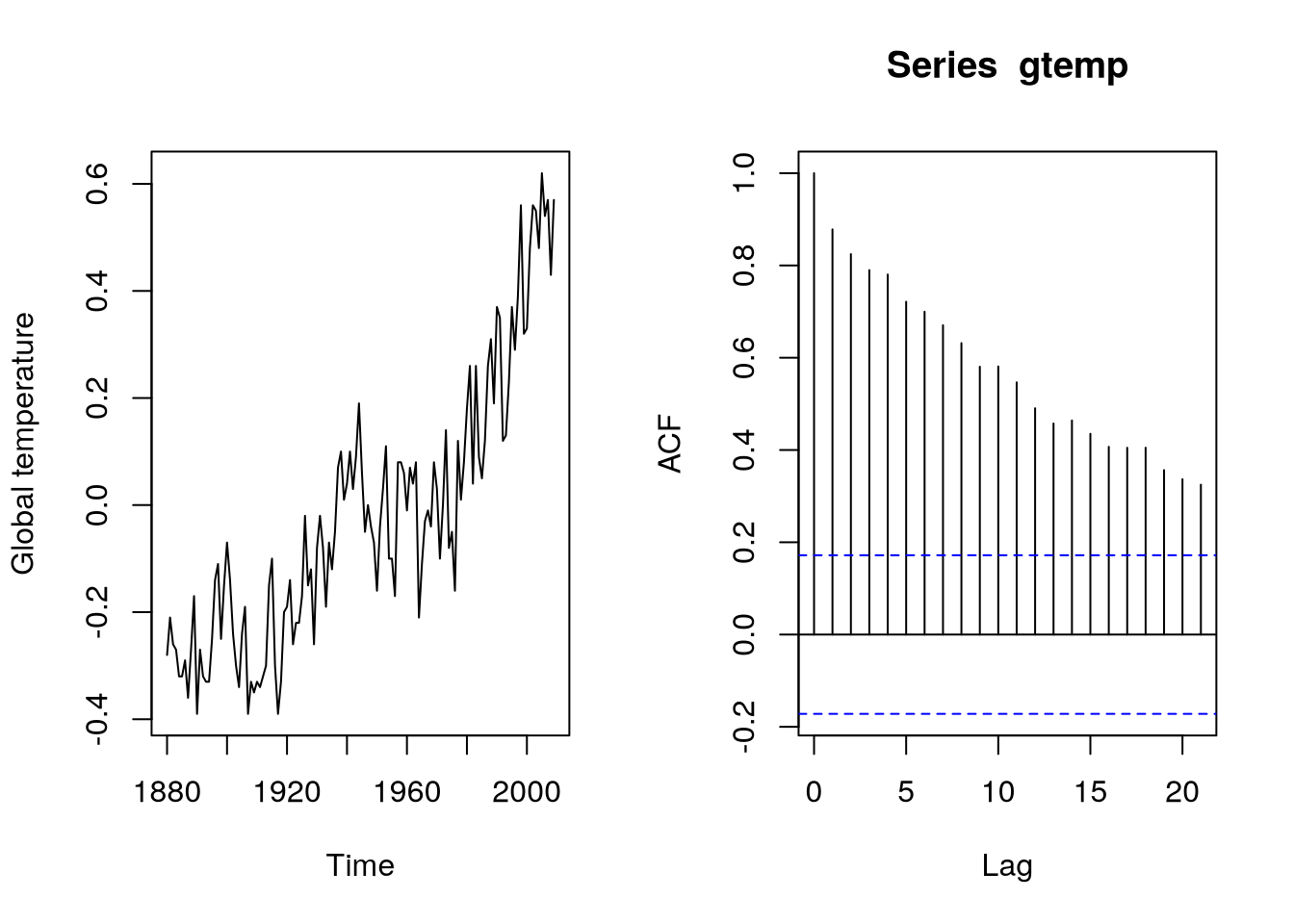
data(gtemp,package="astsa")
par(mfrow=c(1,2))
plot(gtemp,ylab="Global temperature")
acf(gtemp)10 ARIMA, Seasonal ARMA and SARIMA Models
10.1 ARIMA models
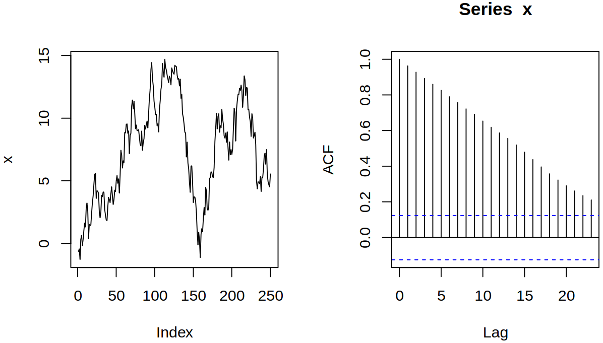
One ARIMA model that we can see is the random walk \(\ARmod{1}\), i.e. \(\rX_t = \vf_1 \rX_{t-1} + \rve_t\), with \(\vf_1 = 1\), thus \[ \rX_t = \rX_{t-1} + \rve_t = \sum_{j = 1}^t \rve_t, \quad t = 1, 2, \dots \]
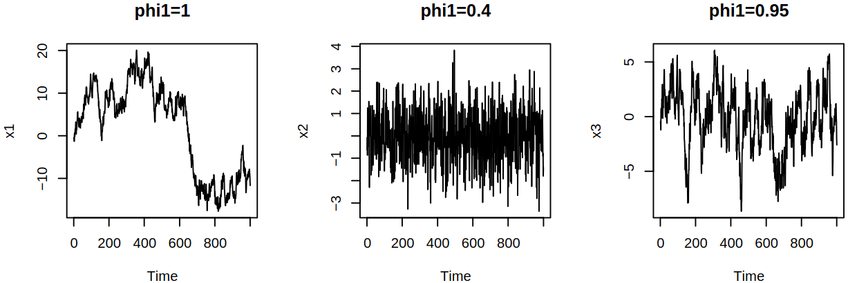
What’s more, we can compare different AR models and notice the differences in their scales, stationarity vs increasing variance and stable behavior vs temporary, transient trends.
As we have discussed before, the correlogram of the random hints (falsely) at a complicated autocorrelation structure (remember that it is misused in this case).
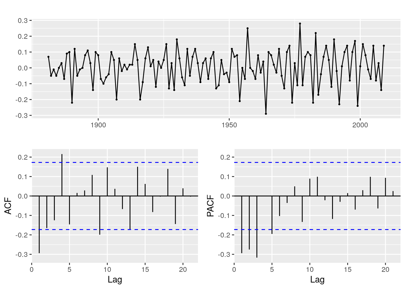
We can see the same behavior in global temperature data, which features similar temporary stochastic trends and even the acf is a look-alike.
10.1.1 Non-stationarity of random walk
Recall that the random walk \[ \rX_t = \rX_{t-1} + \rve_t = \sum_{j = 1}^t \rve_t, \quad t = 1, 2, \dots \] has mean \(\expect X_t = \expect \sum_{j = 1}^n \ve_j = 0\) and \[\begin{gather} \acov(t,t) = \Variance{\sum_{j = 1}^t \rve_j} = t\sigma^2 \\ \acov(s,t) = \Expect{\sum_{j = 1}^s \rve_j \sum_{j = 1}^t \rve_j} = \min(s,t) \sigma^2. \end{gather}\]
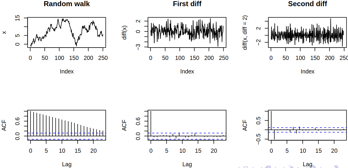
Notice, that the random walk is not stationary but the difference \[ \rX_t - \rX_{t_1} = \rve_t \] is a white noise sequence, hence it is stationary. This suggests that differencing could lead to stationarity.
10.1.2 Differencing time series
Let us define the first difference as \[ \diff \rX_t = \rX_t - \rX_{t-1} = \rX_t - \backs \rX_t = (1 - \backs) \rX_t \] and \(d\)-th difference \[ \diff^d \rX_t = \diff \dots \diff \rX_t = (1 - \backs)^d \rX_t. \] One can realize that differencing
- preserves stationarity: if \(\rX_t\) is stationary, then \((1 - \backs)^d \rX_t\) is also stationary;
- introduces stationarity:
- with deterministic trends: if \(\mu_t\) is a polynomial of order \(d\) and \(\rX_t\) is stationary, then \((1 - \backs)^d (\mu_t + \rX_t)\) is stationary (with constant mean);
- with stochastic trend: random walk becomes stationary after differencing.
Now although differencing may lead to stationarity, it can also give rise to complicated covariance structure if overused. One should consider the principle of parsimony which says that models should be as simple as possible (but not any simpler).
10.1.3 ARIMA model
Definition 10.1 A process \(\rX_t\) is said to be \(\ARIMA{p}{d}{q}\) (integrated ARMA) if \(\diff^d \rX_t = (1 - \backs)^d \rX_t\) is \(\ARMA{p}{q}\).
We shall again use the notation \[ \ArPoly{\backs}(1 - \backs)^d \rX_t = \maPoly(\backs) \rve_t, \] then one can realize that random walk is \(\ARIMA{0}{1}{0}\), or \(\mathrm I(1)\). If the underlying model is ARMA plus mean (instead of just ARMA), i.e., \(\Expect{\diff^d \rX_t} = \mu\), then \(\arPoly{\backs}(\diff^d \rX_t - \mu) = \MaPoly{\backs} \rve_t\), hence \[ \ArPoly{\backs}(1 - \backs)^d \rX_t = \delta + \maPoly(\backs) \rve_t, \] where \(\delta = \mu (1 - \vf_1 - \dots - \vf_p)\). Also, in this case \(\diff^d \rX_t - \mu = \diff^d (\rX_t - \mu t^d / d!)\), i.e., \(\rX_t\) has a polynomial trend. Now consider the following example showcasing the first difference on global temperature data.
10.1.4 Estimating ARIMA models
Clearly, after differencing \(d\) times, we obtain \(\ARMA{p}{q}\) from \(\ARIMA{p}{d}{q}\). Then we can estimate the coefficients, mean and white noise variance of the differenced process by methods for ARMA models (maximum likelihood estimation, conditional least squares etc.). Also, we do not need to center the ARIMA process, as differencing will remove additive constants, see \[ \diff(\rX_t - a) = \diff \rX_t. \] Let now \(\rY_t = \diff^d \rX_t\) be an ARMA model. We can then obtain forecasts of \(\rY_t\) by methods for ARMA processes. Forecasts of \(\rX_t\) can then be obtained by “anti-differencing” – consider \(d = 1\), then
- we have observed data until time \(n\);
- we predict \(\rY_{n+1}\) by \(\estim \rY_{n+1}\);
- since \(\rX_{n+1} = \rX_n + \rY_{n+1}\), predict \(\rX_{n+1}\) by \(\estim \rX_{n+1} = \rX_n + \estim \rY_{n+1}\);
- Predict \(\rY_{n+2}\) by \(\estim \rY_{n+2}(n)\);
- Since \(\rX_{n+2} = \rX_{n+1} + \rY_{n+2}\), predict \(\rX_{n+2}\) by \[ \estim \rX_{n+2} (n) = \estim \rX_{n+1} + \estim \rY_{n+2}(n) = \rX_n + \estim \rY_{n+1} + \estim \rY_{n+2}(n); \]
- etc.
Example 10.1 (Random walk with drift) Consider random walk \[ \rX_t = \delta + \rX_{t-1} + \rve_t, \quad \text{i.e.} \quad \rY_t = \diff \rX_t = \delta + \rve_t \] with \(\rX_0 = 0\). We shall also have observed data \(\rX_1, \dots, \rX_n\) and compute one-step-ahead forecast (which is a projection on \(\linspace{1, \rX_1, \dots, \rX_n}\)) \[ \estim \rX_{n+1} = \BLP_n \rX_{n+1} = \BLP_n(\delta + \rX_n + \rve_{n+1}) = \delta + \rX_n. \] Two-step-ahead forecast has form \(\estim \rX_{n+2}(n) = \delta + \estim\rX_{n+1} = 2\delta + \rX_n\) and similarly \(m\)-step-ahead forecast goes like \(\estim \rX_{n+m}(n) = m \delta + \rX_n\). Compared with stationary \(\ARmod{1}\), \(\rX_t = \delta + \vf_1 \rX_{t-1} + \rve_t\) with \(\absval{\vf_1} < 1\), we see (by successively projecting on the past until \(n + m - 1, n+m - 2, \dots, n\) and using \(\mu = \delta / (1 - \vf_1)\)) that \[ \estim \rX_{n+m} (n) = \delta \frac {1- \vf_1^m} {1 - \vf_1} + \vf_1^m \rX_m = \mu + \vf_1^m (\rX_n - \mu), \] from which we get different asymptotic behavior (as \(m \to \infty\)):
- straight line vs constant;
- persistent vs vanishing effect on \(\rX_n\).
Now to obtain prediction errors, recall that \[ \rX_n = n \delta + \sum_{j = 1}^n \rve_j \quad \& \quad \rX_{n+m} = m\delta + \rX_n + \sum_{j = n+1}^{n+m} \rve_j \] and the prediction error is \[ \Expect{\rX_{n+m} - \estim \rX_{n+m}(n)}^2 = \Expect{\sum_{j = n+1}^{n+m} \rve_j}^2 = m\sigma^2. \] Also remember that for a stationary \(\ARmod{1}\) model, we have seen that \[ \Expect{\rX_{n+m} - \estim \rX_{n+m}(n)}^2 = \sigma^2 \frac{1 - \vf_1^{2m}} {1 - \vf_1^2}, \] which also shows different asymptotic behavior (as \(m \to \infty\)) of growing (or diverging) vs converging prediction errors.
Example 10.2 (\(\mathrm{IMA}(1,1)\) and exponential smoothing) Consider an \(\ARIMA{0}{1}{1}\), or \(\mathrm{IMA}(1,1)\) model, \[ \rX_t = \rX_{t-1} + \rve_t - \lambda \rve_{t-1} \] with \(\absval{\lambda} < 1\), for \(t = 1,2, \dots\) and \(\rX_0 = 0\). Now \[ \rX_t - \rX_{t-1} = \rve_t - \lambda \rve_{t-1} \] has an invertible representation \(\sum_{j = 0}^\infty \lambda^j\backs^j(\rX_t - \rX_{t-1}) = \rve_t\). Then for large \(t\) we can approximate (set \(\rX_t = 0\), \(t \leq 0\)) \[ \rX_t = \sum_{j = 1}^\infty (1 - \lambda) \lambda^{j-1} \rX_{t-j} + \rve_t. \] Now approximate one-step prediction by \[ \infEstim \rX_{n+1} = \sum_{j = 1}^\infty (1 - \lambda) \lambda^{j-1} \rX_{n+1-j} = (1 - \lambda) \rX_n + \lambda \infEstim \rX_n. \] Thus the forecast is a linear combination of the old forecast and the new observation, which is also called exponentially weighted moving average (EWMA).
This is then equivalent to Holt’s linear method, as we’ve seen before.
10.2 Seasonal ARMA models
Seasons are important in applications: economics, environment, etc. We have so far seen
- Classical decomposition;
- Seasonal indicators, harmonic functions;
- STL;
- Holt–Winters,
but often, there is a strong dependence on the past at multiples of some seasonal lag \(s\) (e.g., \(s = 12\) months). At the same time, there is some variation (beyond fixed seasonal effects) Hence our goal becomes to incorporate this into ARMA models
One can realize that seasonal lags correspond to powers of the backshift operator \(\backs^{js}\), e.g. \(\backs^{12}\rX_t = \rX_{t-12}\) is the value one year ago for monthly time series. We can then define the seasonal autoregressive operator \[ \arPoly^*(\backs^s) = 1 - \vf_1^* \backs^s - \vf_2^* \backs^{2s} - \dots - \vf_P^* \backs^{Ps} \] and seasonal moving average operator \[ \maPoly^*(\backs^s) = 1 + \tht_1^* \backs^s + \dots + \tht_Q^* \backs^{Qs}, \] from which we obtain pure seasonal ARMA models by combining \[ \arPoly^*(\backs^s) \rX_t = \maPoly^*(\backs^s)\rve_t \]
Note that pure seasonal models only include powers of \(\backs^s\), but the dependence at other than seasonal lags is also needed (e.g., previous month). Thus we combine both seasonal and non-seasonal (typically shorter lag) dependence to get multiplicative seasonal ARMA model \[ \arPoly(\backs)\arPoly^*(\backs^s) \rX_t = \maPoly(\backs)\maPoly^*(\backs^s)\rve_t. \]
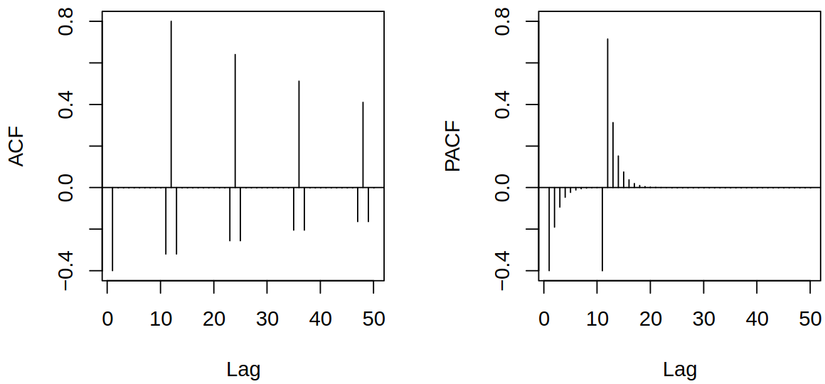
As an example, we can take a look at \(\sARMA{0,1}{0,1}{12}\) \[ \rX_t = 0.8 \rX_{t-12} + \rve_t - 0.5 \rve_{t-1}. \]
10.2.1 Estimation and prediction
Clearly, the seasonal ARMA model is an ARMA model with special AR and MA polynomials, which puts constraints on the coefficients (thus reduces free parameters), e.g. \[ (1 - \vf_1^* \backs^{12})(1 - \vf_1\backs) \rX_t = \rve_t \] is an \(\ARmod{13}\) model but has only two parameters. Estimation procedures are then similar to non-seasonal ARMA (MLE etc.) but they exploit these parameter constraints (which gives us fewer parameters to estimate). Lastly, prediction is similar as with the usual ARMA model.
10.3 Seasonal ARIMA models
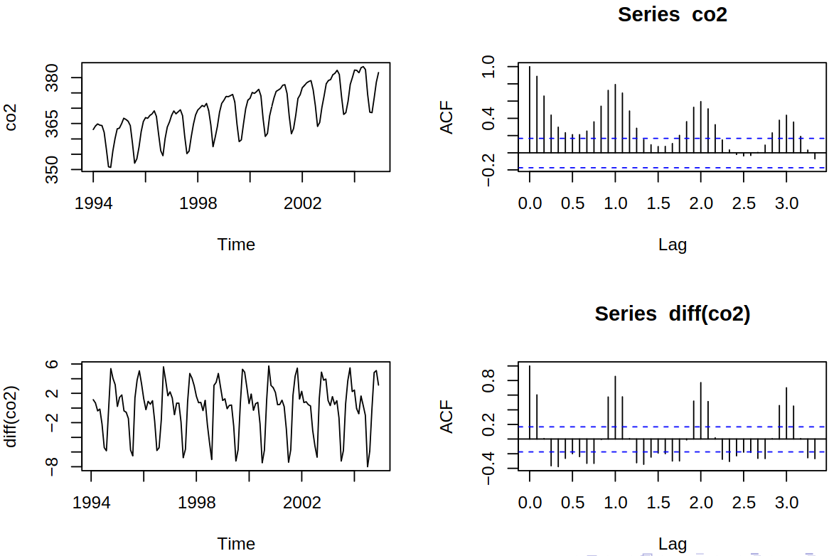
Recall the \(\text{CO}_2\) series, see Example 5.2.
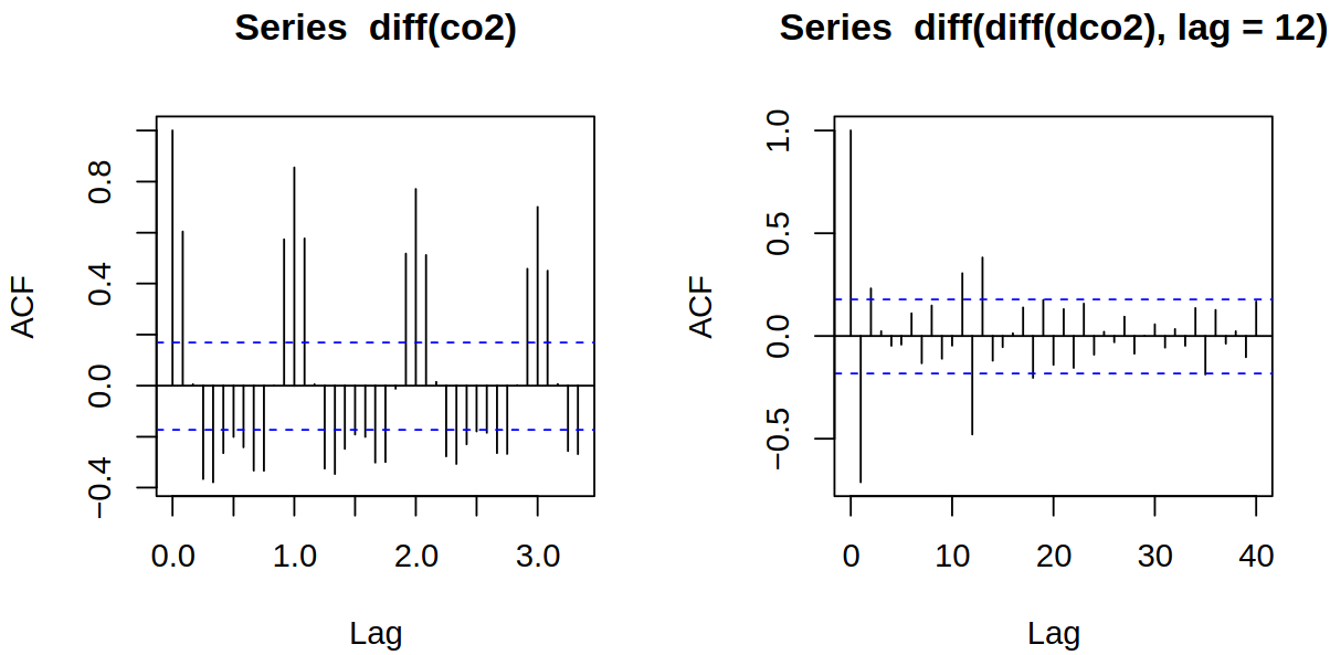
Now by multiple differencing, we get Figure 10.1, where we can see that while autocorrelation \(\acf\) at seasonal lags decreases slowly, with the seasonal differencing we get a fast decrease.
10.3.1 Multiplicative seasonal ARIMA models
Seasonal differencing is defined by \[ (1 - \backs^s) \rX_t = \rX_t - \rX_{t-s}, \] e.g. \((1 - \backs^{12}) \rX_t = \rX_t - \rX_{t - 12}\) (beware, it is not \((1 - \backs)^{12} = \diff^{12}\)). Higher-order seasonal differences are then \((1 - \backs^s)^D X_t\). Now we can combine seasonal differencing, ordinary differencing, seasonal and ordinary AR and MA modeling.
Definition 10.2 (SARIMA model) The multiplicative seasonal autoregressive integrated moving average (SARIMA) model is given by \[ \arPoly^*(\backs^s)\arPoly(\backs)(1 - \backs^s)^D (1 - \backs)^d \rX_t = \delta + \maPoly^*(\backs^s)\maPoly(\backs) \rve_t, \] where \(\rve_t\) is white noise and \(\arPoly, \arPoly^*, \maPoly, \maPoly^*\) are polynomials of order \(p, P, q, Q\) respectively, which we denote by \(\SARIMA{p,d,q}{P,D,Q}{s}\).
Example 10.3 (\(\SARIMA{0,1,1}{0,1,1}{12}\)) Consider a model given by \[ (1 - \backs^{12})(1 - \backs) \rX_t = \maPoly^*(\backs^{12}) \maPoly(\backs)\rve_t, \] where \(\maPoly^*(\backs^{12}) = 1 + \tht_1^* \backs^{12}\) and \(\maPoly{\backs} = 1 + \tht_1 \backs\). By expanding and rearranging we get \[ \rX_t = \rX_{t-1} + \rX_{t-12} - \rX_{t-13} + \rve_t + \tht_1 \rve_{t-1} + \tht_1^* \rve_{t-12} + \tht_1 \tht_1^* \rve_{t-13}. \] Due to the multiplicative nature of the model, the coefficient at \(\rve_{t-13}\) is \(\tht_1 \tht_1^*\) rather than a free parameter.
10.3.2 Estimation and forecasting or SARIMA models
First, one should difference the series according to the model (take \(d\) ordinary and \(D\) seasonal differences), then estimate the corresponding SARMA model (i.e., ARMA with a special form of the polynomials) and lastly forecast the differenced series and anti-difference it.
10.4 Further reading
10.4.1 Long seasonal periods
SAR(I)MA models are suitable for short periods, e.g., 12 (or 4) for monthly (or quarterly) data within years, 7 for daily data within weeks, 24 for hourly data within days etc. Long periods, e.g., 365 for daily data within years, are not meaningful practically and not supported by standard software. In such cases, one should use harmonic (or other periodic) functions instead, see forecasting with long seasonal periods.
10.4.2 Constants, trends,… in integrated models
In non-differenced models, one can include the intercept (constant vertical shift of the series). In the case of first-order differencing, the vertical shift is not estimable (differencing removes it) but the slope of the linear trend is. Similarly, under differencing of order \(d\), the vertical shift of the series by a polynomial of degree \(< d\) is not estimable; shift by \(t^d\) is estimable but not permitted for \(d > 1\) by forecast::Arima (dangerous extrapolation), for more information see constants and ARIMA models in R.
Also, the regression matrix in xreg (for regression plus AR(I)MA errors) must not be collinear with the vertical shift and must not contain non-estimable terms (those whose \(d\)-th difference is zero)

