data(gtemp,package="astsa")
plot(gtemp,type="o",ylab="Global temperature")5 Regression Methods for Deterministic Components
5.1 Linear regression models
Observable processes follow some deterministic patterns but randomly deviate from them. From these assumptions, we may write our time series as a model plus noise decomposition \[ \rnd X_t = \text{Deterministic}_t + \text{Stochastic}_t. \]
Furthermore, the deterministic part can be modeled as follows \[ \text{Deterministic}_t = \text{Trend}_t + \text{Seasonality}_t \;({}+ \text{OtherVariablesEffects}_t) \] and the stochastic component as (we will see models of this kind, e.g. ARMA, later) \[ \text{Stochastic}_t = \text{PredictableVariation}_t + \text{WhiteNoise}_t. \]
The above decompositions are schematic, and not always applicable. (non-stationarity, non-linearity, changing variability etc.)
We shall now look at parametric modeling of the deterministic part.
5.1.1 Examples
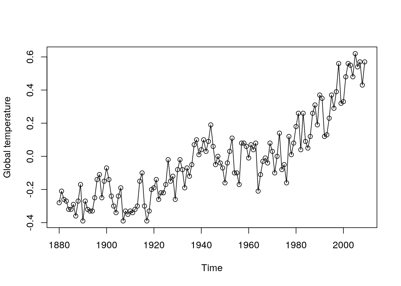
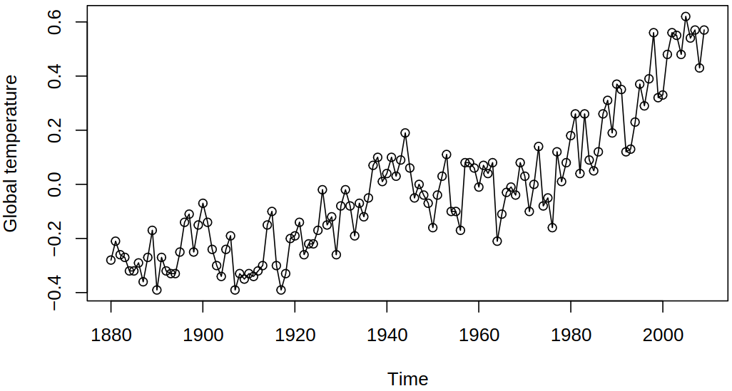
Example 5.1 (Annual global temperature series) With the following code, we can plot Figure 5.1, where a possible monotonic trend (linear, maybe quadratic) can be seen.
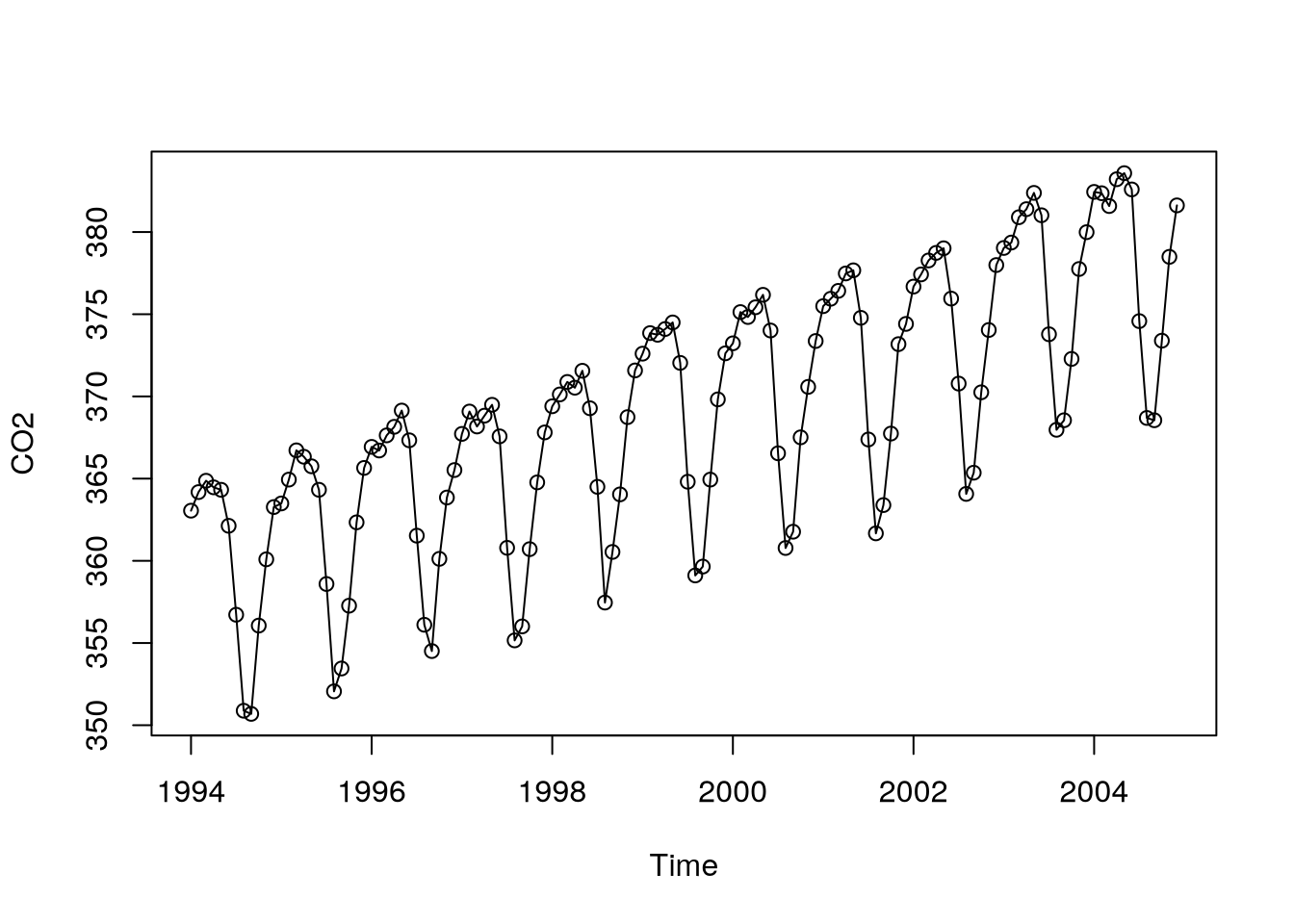
Example 5.2 (Monthly carbon dioxide levels) Now, consider the following time series, in which one can see a clear monotonic trend (linear) and seasonality.
5.1.2 Linear models for trends in time
Consider a model \[ \rnd X_t = \mu_t + \rnd U_t, \] where \(\mu_t = \expect \rnd X_t\) is the mean, \(\rnd U_t\) are residuals \(\expect \rnd U_t = 0\). Models for the trend should be simple, model only obvious trends (such as monotonic) and seasonality. Unclear/varying/transient features (stochastic trends) are often handled by differencing, for example
- linear trend: \(\mu_t = \beta_0 + \beta_1 t\);
- quadratic trend: \(\mu_t = \beta_0 + \beta_1 t + \beta_2 t^2\).
We usually do not use higher-order polynomials (a complicated graph of the whole process may likely be due to stochastic trends).
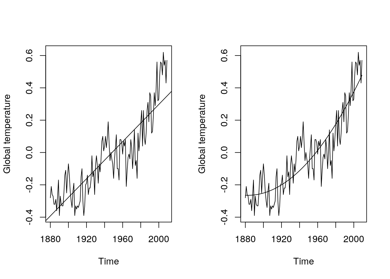
Example 5.4 As introduced earlier, we can use the following code to model with deterministic components the Example 5.1 data:
gtemp.m1 = lm(gtemp~time(gtemp))
gtemp.m2 = lm(gtemp~time(gtemp)+I(time(gtemp)^2))
par(mfrow=c(1,2))
plot(gtemp,ylab="Global temperature")
abline(gtemp.m1)
plot(gtemp,ylab="Global temperature")
lines(as.vector(time(gtemp)),fitted(gtemp.m2))Now, we shall look at the summary statistics of the used models.
summary(gtemp.m2)
Call:
lm(formula = gtemp ~ time(gtemp) + I(time(gtemp)^2))

Residuals:
      Min        1Q    Median        3Q       Max
-0.300105 -0.080650  0.004134  0.074619  0.280003

Coefficients:
                   Estimate Std. Error t value Pr(>|t|)
(Intercept)       1.647e+02  2.916e+01   5.647 1.02e-07 ***
time(gtemp)      -1.752e-01  3.000e-02  -5.840 4.12e-08 ***
I(time(gtemp)^2)  4.653e-05  7.714e-06   6.032 1.65e-08 ***
---
Signif. codes:  0 '***' 0.001 '**' 0.01 '*' 0.05 '.' 0.1 ' ' 1

Residual standard error: 0.1108 on 127 degrees of freedom
Multiple R-squared:  0.8065,    Adjusted R-squared:  0.8035
F-statistic: 264.7 on 2 and 127 DF,  p-value: < 2.2e-16
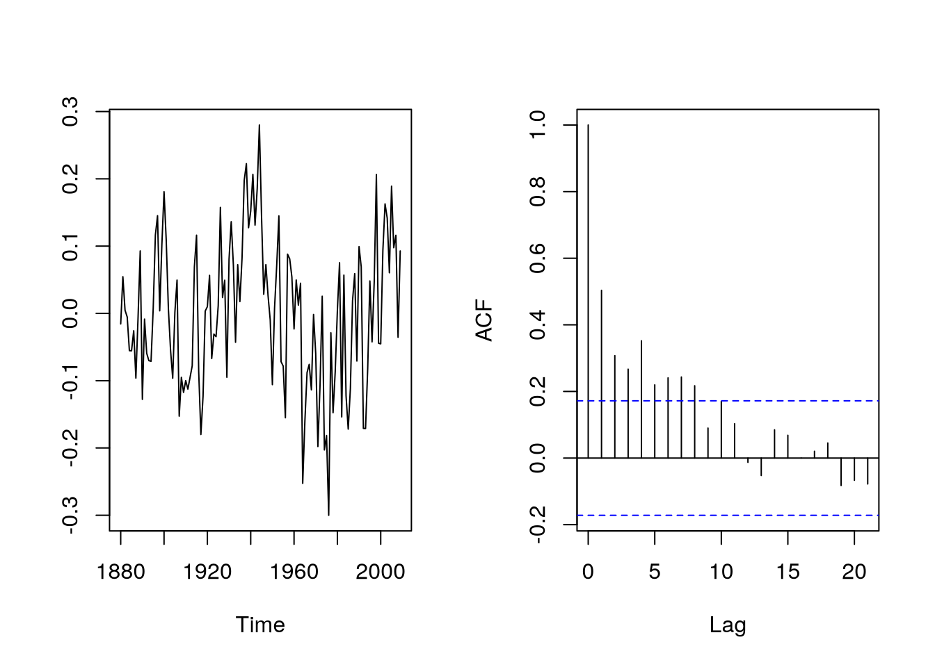
But can we trust these standard errors, confidence intervals and \(p\)-values? In the theory of linear regression models, we mostly assumed independence. We can look at the residuals
par(mfrow=c(1,2))
plot(as.vector(time(gtemp)),
    resid(gtemp.m2),
    type="l",
    xlab="Time",
    ylab=""
)
acf(resid(gtemp.m2),
    main=""
)As can be seen in Figure 5.3, the residuals are strongly autocorrelated and the standard errors, \(p\)-values are probably incorrect (they are computed under the assumption of iid errors).
5.1.3 Linear models for trends and seasonality
Again, consider a model \(\rnd X_t = \mu_t + \rnd U_t\), where \(\mu_t = \expect \rnd X_t\) is the mean, \(\rnd U_t\) are residuals \(\expect \rnd U_t = 0\). Now we can include the seasonal effect. Consider \(s\) seasons (e.g. \(s = 12\)), each having its own level. Then the model with linear trend and seasonal indicators is of form \[\begin{align*} \mu_t &= \beta_0 + \beta_1 t + \sum_{j = 2}^s \alpha_j \indicator{t=ks+j} \\ &= \begin{cases} \beta_0 + \beta_1 t, & t = 1, s + 1, 2s + 1, \dots \\ \beta_0 + \beta_1 t + \alpha_2, & t = 2, s + 2, 2s + 2, \dots \\ \vdots & \\ \beta_0 + \beta_1 t + \alpha_s, & t = s, 2s, 3s, \dots, \end{cases} \end{align*}\] where season \(1\) is the reference level and \(\alpha_2, \dots, \alpha_s\) are the differences against it.
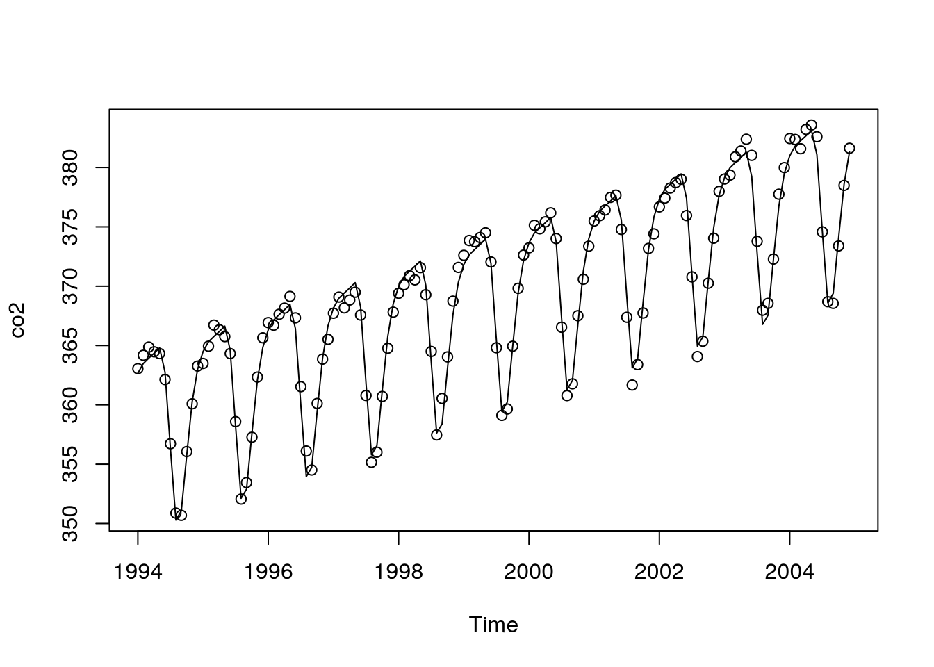
Using the following code, we get the model seen in Figure 5.4.
mth = factor(cycle(co2))
co2.m1 = lm(co2~time(co2)+mth)
plot(co2,type="p")
lines(as.vector(time(co2)),fitted(co2.m1))Or we can consider other equivalent models.
lm(co2~time(co2)+mth)
Call:
lm(formula = co2 ~ time(co2) + mth)

Coefficients:
(Intercept)    time(co2)         mth2         mth3         mth4         mth5
 -3290.5412       1.8321       0.6682       0.9637       1.2311       1.5275
       mth6         mth7         mth8         mth9        mth10        mth11
    -0.6761      -7.2851     -13.4415     -12.8205      -8.2604      -3.9277
      mth12
-1.3367 lm(co2~time(co2)-1+mth)
Call:
lm(formula = co2 ~ time(co2) - 1 + mth)

Coefficients:
time(co2)       mth1       mth2       mth3       mth4       mth5       mth6
    1.832  -3290.541  -3289.873  -3289.577  -3289.310  -3289.014  -3291.217
     mth7       mth8       mth9      mth10      mth11      mth12
-3297.826  -3303.983  -3303.362  -3298.802  -3294.469  -3291.878
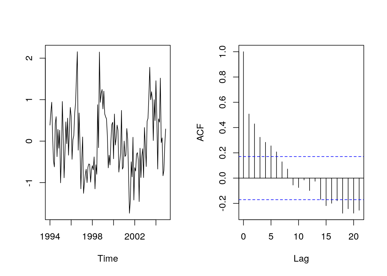
Also, we can look at the residuals and last, but not least, we can plot fitted values of our \(CO_2\) model.
par(mfrow=c(1,2))
plot(as.vector(time(co2)),
    resid(co2.m1),
    type="l",
    xlab="Time",
    ylab=""
)
acf(resid(co2.m1),
    main=""
)
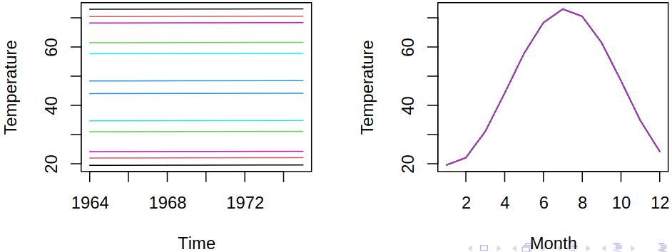
Notice that there are parallel monthly lines with different distances and parallel (almost equidistant) profiles within years
5.1.4 Seasonality via harmonic components
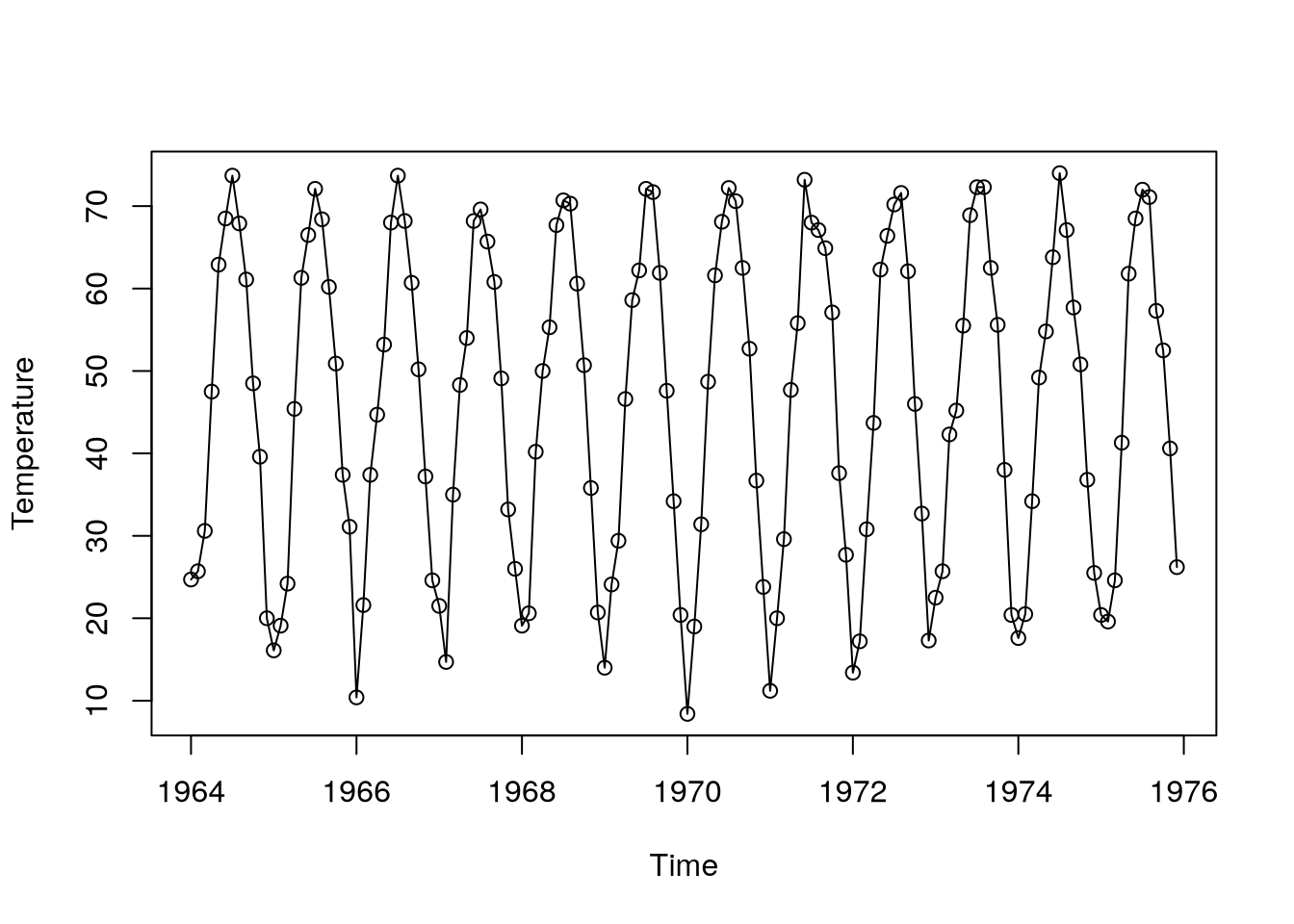
Consider the following time series from Example 5.3.
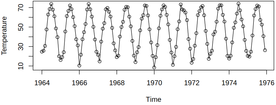
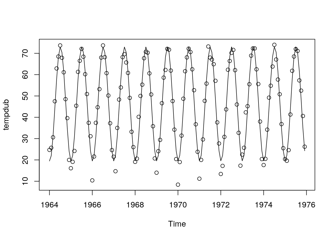
Here, waves look like cosines (unlike in the \(\text{CO}_2\) series), so our idea might be to model the deterministic component with a cosine wave with known frequency (e.g., \(f = \frac 1 {12}\)) and unknown amplitude and phase \[ \mu_t = \beta_0 + \beta_1 t + a \cos \brackets{2\pi f t + \vf}. \]
Now, we have to estimate intercept \(\beta_0\), slope \(\beta_1\), amplitude \(a\), phase \(\vf\), but the model is non-linear in \(\vf\), which would be difficult to estimate. From trigonometry we get \[ a \cos \brackets{2\pi f t + \vf} = \alpha_1 \cos(2 \pi f t) + \alpha_2 \sin(2 \pi f t), \] where \(\alpha_1 = a \cos(\vf)\), \(\alpha_2 = - \sin(\vf)\). This transforms our model to \[ \mu_t = \beta_0 + \beta_1 t + \alpha_1 \cos(2 \pi f t) + \alpha_2 \sin(2 \pi f t) \] and this model is linear in parameters (and we have 4 parameters to estimate: \(\beta_1, \beta_2, \alpha_1, \alpha_2\)). It is good to use known, logical frequencies for deterministic modeling (e.g. \(f = 1/12\)). Compared with seasonal indicators we have less flexibility, more restrictive, but also fewer parameters.
More components, continuum of components, spectral analysis, relative importance of components, periodogram, FFT, random cosine wave stationary model, …
Example 5.5 The derived model yields Figure 5.5
tempdub.harm = lm(tempdub~time(tempdub)
    +cos(2*pi*time(tempdub))
    +sin(2*pi*time(tempdub))
)
plot(tempdub,type="p")
lines(as.vector(time(tempdub)),
    fitted(tempdub.harm)
)We can now look at the fitted values in the harmonic model for monthly temperatures.
tempdub.harm
Call:
lm(formula = tempdub ~ time(tempdub) + cos(2 * pi * time(tempdub)) +
    sin(2 * pi * time(tempdub)))

Coefficients:
                (Intercept)                time(tempdub)
                   23.85687                      0.01138
cos(2 * pi * time(tempdub))  sin(2 * pi * time(tempdub))
                  -26.70699                     -2.16621
5.2 Regression estimators and their properties
Consider a model \(\rnd X_t = \mu_t + \rnd U_t\) with \[ \mu_t = \sum_{j = 1}^p \vi \beta_j Z_{tj}, \quad t = 1,2,\dots \]
Presume we have observations at \(t = 1, \dots, n\). We write \(\mu = \vi Z \vi \beta\) in matrix notation (\(\vi Z\) is \(n \times p\), assume full rank \(p\)). Typically, columns of \(\vi Z\) are \(\vi 1\) (intercept), \(t\) (linear trend), possibly \(t^2\), seasonal indicators or sines and cosines, and maybe other explanatory variables (assume non-random). Now our goal is to estimate \(\vi \beta\) by (ordinary) least squares (OLS or LS): minimize \[ \norm{\vr X - \vi Z \vi \beta}_2^2 = \sum_{t = 1}^n (\rnd X_t - \vi Z_t\Tr\vi \beta)^2. \]
Although the textbook solution is \[ \estim{\vi \beta} = (\vi Z\Tr \vi Z)^{-1} \vi Z\Tr \vr X, \] we typically use QR-decomposition, i.e. we factorize \(\vi Z = \vi Q \vi R\), where \(\vi Q\) (\(n \times p\)) has orthonormal columns and \(\vi R\) is (\(p \times p\)) upper triangular, so the objective becomes
\[ \norm{\vr X - \vi Z \vi \beta}_2^2 = \norm{\vr X - \vi {QR\beta}}^2_2 = \norm{\vr X - \vi{Q \gamma}}_2^2, \] where \(\vi \gamma = \vi R \vi \beta\). Since the transformation \(\vi \gamma = \vi R \vi \beta\) is one-to-one (\(\vi R\) has full rank), we can first minimize \(\norm{\vr X - \vi{Q \gamma}}_2^2\) over \(\vi \gamma \in \R^p\) to get \(\estim{\vi \gamma}\) and the solve \(\vi R \vi \beta = \estim{\vi \gamma}\) to get \(\estim{\vi \beta}\).
Minimizing \(\norm{\vr X - \vi Q \vi \gamma}_2^2\) is easy because \(\vi Q\) has orthonormal columns, thus \(\estim{\gamma}_j = \scal {\vr X} {\vi Q_{\cdot, j}}\). Also, solving \(\vi R \vi \beta = \estim{\vi \gamma}\) is cheap because \(\vi R\) is triangular (back-substitution can be used).
5.2.1 Properties of the OLS estimator
Surely \(\estim {\vi \beta}\) is unbiased (in spite of ignoring dependence) \[ \expect \estim{\vi \beta} = (\vi Z\Tr \vi Z)^{-1} \vi Z\Tr (\expect \vr X) = \vi \beta. \]
Moreover, if \(\vr U\) is stationary with \(\cov \vr U = \covMat = \sigma^2 \vr R\), the variance is \[ \begin{aligned} \variance \estim{\vi \beta} &= (\vi Z\Tr \vi Z)^{-1} \vi Z\Tr \covMat \vi Z (\vi Z\Tr \vi Z)^{-1} \\ &= \sigma^2 (\vi Z\Tr \vi Z)^{-1} \vi Z\Tr \vr R \vi Z (\vi Z\Tr \vi Z)^{-1}. \end{aligned} \tag{5.1}\]
Recall the form \(\variance \estim{\vi \beta} = \sigma^2 (\vi Z\Tr \vi Z)^{-1}\) for \(\vr R = \ident\) for the iid case in (5.1).
Thus the usual standard errors, confidence intervals, and \(p\)-values will be incorrect under autocorrelation. Often, the inference about the deterministic components is not the goal, we just want to remove the trend and focus on the stochastic part, then move on to prediction.
One possible remedy could be the sandwich estimators \[
\variance \estim{\vi \beta} = (\vi Z\Tr \vi Z)^{-1} \vi Z\Tr \estim{\covMat} \vi Z (\vi Z\Tr \vi Z)^{-1}
\] where \(\estim{\covMat}\) is an estimator such that \(\vi Z\Tr \estim{\covMat} \vi Z / n\) consistently estimates the limit of \(\vi Z\Tr \covMat \vi Z / n\) (similar to long-run variance in mean estimation), see sandwich::vcovHAC.
5.2.2 Generalized least squares
Surely, we can use the (assumed) correct covariance matrix derived earlier for estimation. Then we get generalized least squares (GLS), where we solve \[ \min_{\vi \beta} (\vr X - \vi Z \vi \beta)\Tr \covMat^{-1}(\vr X - \vi Z \vi \beta), \] which is motivated by
- Gaussian likelihood: maximize the likelihood for \(\vr X \sim \normalDist_n(\vi Z \vi \beta, \covMat)\) \[ (2\pi)^{-k/2} (\det \covMat)^{-1/2} \exp \brackets{-(\vr X - \vi{Z\beta})\Tr \covMat^{-1}(\vr X - \vi {Z\beta})/2}; \]
- Standardization and OLS: surely \(\covMat^{-1/2} \vr X\) has mean \(\covMat^{-1/2}\vi Z \vi \beta\) and variance \(\covMat^{-1/2}\covMat \covMat^{-1/2} = \ident\), hence \(\covMat^{-1/2} \vr X\) are uncorrelated. As such we can solve the OLS minimization. \[ \begin{aligned} \brackets{\covMat^{-1/2} \vr X- \covMat^{-1/2}\vi{Z\beta}}\Tr &\brackets{\covMat^{-1/2} \vr X- \covMat^{-1/2}\vi{Z\beta}} \\ &= \brackets{\vr X - \vi {Z\beta}}\Tr \covMat^{-1/2} \brackets{\vr X - \vi {Z\beta}}. \end{aligned} \]
All in all, the textbook solution is now \[ \estim{\vi \beta} = \brackets{\vi Z\Tr \covMat^{-1} \vi Z}^{-1} \vi Z\Tr \covMat^{-1} \vr X. \]
Note that the difficulty with GLS is the need to know \(\covMat\), but we can specify a model for \(\covMat\) (or \(\vr R\)) up to some parameters and estimate both \(\vi \beta\) and the parameters of \(\covMat\) by maximum likelihood. As an example, for moving average errors, one can use a banded matrix.
How do we know that the correlation model was correctly specified? The residuals should look like white noise (in particular, no correlation). The function gls in the R package nlme can do this estimation but it is primarily designed for something else (grouped data), we will see tools that are more appropriate for time series
5.2.3 Transformations
Some of the common problems – think heteroskedasticity (e.g. variance increases with mean), non-linearity, non-stationarity or non-normality (skewness) – can be addressed using transformations to make residuals look stationary and normal. After transforming our data, we then fit the regression models to the transformed series. Most commonly, a \(\log\) or square root transformations are used, e.g. \[ \rnd X_t = m_t \rnd U_t \mapsto \log \rnd X_t = \log (m_t) + \log (\rnd U_t) \] where a non-stationary, heteroskedastic series is transformed to a trend part plus stationary part (if \(\rnd U_t\) is stationary). In general, the \(\log\) transformation isn’t the only possible one in this case (that gives us linearity and stationarity). Consider a transformation \(g\) such that \[ \rnd X_t \mapsto g(\rnd X_t) = m_t^* + \rnd U_t^*, \] where \(g\) may be, for example, the Box-Cox transformation, see Definition 5.1.
Definition 5.1 (Box-Cox Transformation) Let \(\rnd X_t = m_t \rnd U_t\) be a time series and \(g\) the Box-Cox transformation given by \[ g(x) = \frac {x^\lambda - 1} \lambda \] for \(\lambda > 0\) and \(g(x) = \log x\) for \(\lambda = 0\).
Here \(\lambda = 0\) corresponds to a multiplicative transformation and \(\lambda = 1\) to an additive one.
But now a question arises how and when do Box-Cox transformations work? Suppose that \(\rnd X_t > 0\) and that \[ \expect \rnd X_t = \mu_t \quad \& \quad \variance \rnd X_t = \sigma^2 v(\mu_t). \] Now consider the Taylor expansion \[ g(\rnd X_t) \approx g(\mu_t) + g'(\mu_t)(\rnd X_t - \mu_t) \] and compute expectations and variances on both sides to get \[ \expect g(\rnd X_t) \approx g(\mu_t), \quad \variance g(\rnd X_t) \approx g'(\mu_t)^2 \variance \rnd X_t = g'(\mu_t)^2 \sigma^2 v(\mu_t). \]
To further stabilize the variance, i.e. make it independent of the mean, use \(g\) such that \(g'(x) = v^{-\frac 1 2}(x)\). As can be shown, the Box-Cox transformations do this for \(v(x) = cx^{2(1 - \lambda)}\) – in other words when the standard deviation of \(X_t\) is proportional to \(\mu_t^{1 - \lambda}\).
Using this we get a \(\log\) transformation for the variance quadratic in the mean and square root for the variance linear in the mean.
5.3 Nonparametric regression techniques
Consider a time series describing global temperature
Here the “trend” does not really look either quadratic or linear (or simple in any way), but we would still like to estimate the central trajectory and remove the fluctuations. And for this we may use nonparametric smoothing.
Our goal now is to take a time series and “extract” its main shape while removing the noise. Thus, suppose we can decompose the series into \[ \rnd X_t = T_t + \rnd E_t, \tag{5.2}\] where \(T_t\) is the trend component and \(E_t\) are random, irregular fluctuations (noise) and we want to estimate \(T_t\). Previously we used linear regression, e.g. we set \(T_t = a + bt\), but we can allow \(T_t\) to vary more flexibly. Instead of assuming a parametric (e.g., linear) model for the trend, we will estimate it nonparametrically as a general function of \(t\).
This process has many applications, e.g. exploratory analysis, graphics, detrending or simply the preparation for the analysis of the random part.
5.3.1 Moving averages
As mentioned before, our goal is to remove fluctuations and preserve the “central” values of a given time series. Naturally, we can assume that locally the series values fluctuate around a similar level. The fluctuations have a zero mean and as such should cancel out when averaged (locally). Thus we consider a moving average smoother, see Definition 5.2.
Definition 5.2 (Moving average Smoother) Moving average smoother of order \(m = 2k+1\) is a transformed series \[ \estim{\rnd T}_t = \frac 1 m \sum_{j = -k}^k \rnd X_{t+j}, \] or for \(m = 2k\) even, we can use \[ \estim{\rnd T}_t = \frac 1 {2m} \rnd X_{t-k} + \frac 1 m \rnd X_{t-k+1} + \dots + \frac 1 m \rnd X_{t+k-1} + \frac 1 {2m} X_{t+k}. \]
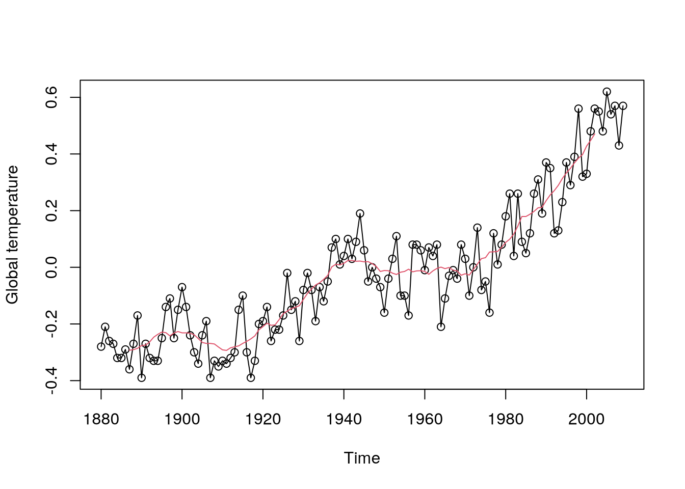
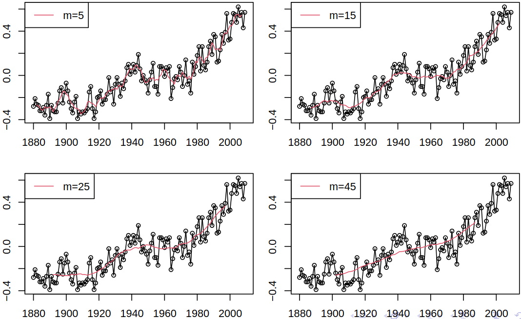
As a terminology side note, “moving average” is used for the above estimator of the trend as well as for the model based on the moving average of white noise. Recall the global temperature time series from Figure 5.6, on which we can demonstrate the moving average smoother, see Figure 5.7.
library(forecast)Registered S3 method overwritten by 'quantmod':
method from
as.zoo.data.frame zoo plot(gtemp,type="o",ylab="Global temperature")
lines(ma(gtemp,15),col=2)Furthermore, we can compare the effect of different orders of the moving average.
5.3.2 Kernel smoothing
The aforementioned moving average smoother, see Definition 5.2, locally averages observations, but all are given the same weight. We could generalize this concept – consider moving weighted averages with weights depending on the proximity to the time point of interest.
Definition 5.3 (Kernel Smoothing (Nadaraya-Watson estimator)) The Kernel smoothing uses \[ \estim{\rnd T}_t = \sum_{i = 1}^n w_i(t)\rnd X_i, \] where the weights \(w_i\) are defined as \[ w_i(t) = \frac{K\brackets{\frac {i-t} h}} {\sum_{j = 1}^n K\brackets{\frac {j-t} h}}. \]
Here \(K\) is a kernel function, e.g. \(K(z) = (2\pi)^{-\frac 1 2} \exp{- \frac {z^2} 2}\), and \(h\) is the bandwidth that controls the smoothness.
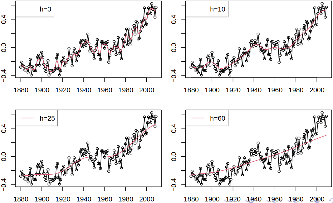
For large \(h\), \(w_i(t)\) is large even when \(i\) is far from \(t\), and thus \(w_i(t)\) is “flat”, averaging relies on distant observations and there is a possibility of over-smoothing.
On the other hand, for small \(h\), \(w_i(t)\) is large only when \(i\) is close to \(t\), and thus \(w_i(t)\) drops quickly. Averaging then depends mainly on nearby observations but under-smoothing is possible.
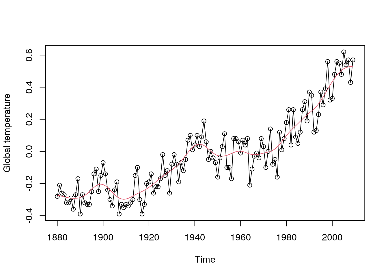
If we again apply this method to our example, see Figure 5.6, we get Figure 5.8.
plot(gtemp,type="o",ylab="Global temperature")
lines(ksmooth(
        time(gtemp),
        gtemp,
        kernel="normal",
        bandwidth=10
    ),
    col=2
)What’s more, we can also compare the effect of bandwidth on the estimate.
As for the properties of the kernel smoother (see Definition 5.3), \(\estim{\rnd T}_t\) in fact estimates the smoothed version of \(T_t\) taken from (5.2) (also see Definition 5.2) and \[ \expect\estim{\rnd T}_t = \sum_{i = 1}^n w_i(t) T_i. \] As \(\estim{\rnd T}_t\) is a linear function of data, the variance of the kernel smoother is easy to find, if the autocovariance \(\acov\) of the series is known (e.g. in iid case). Then \[ \variance \estim{\rnd T}_t = \sum_{i = 1}^n \sum_{j = 1}^n w_i(t) w_j(t) \acov(i,j). \]
In time series analysis, we typically use kernel smoothing as an exploratory technique, when we are not much interested in the standard errors, confidence intervals etc. There is also a bias-variance tradeoff:
- large \(h\) gives us high bias but low variance;
- small \(h\) gives us low bias but high variance.
And while automatic procedures to find the best compromise do exist, they often assume iid errors and risk possible overfitting with positive autocorrelation, i.e., series of similar values.
There are, of course, more advanced kernel smoothing techniques:
- locally polynomial fitting (Nadaraya–Watson is locally constant),
- locally adaptive choice of \(h\) (\(h\) depending on \(t\)),
- etc.
5.3.3 Other smoothing techniques
Although we don’t have the time to explain and show the following methods in this course, one can also use
- Splines
- Express \(T_t\) as a linear combination of spline functions;
- Estimate by least squares – possibly with penalization for “roughness” (to avoid fitting the data instead of the trend);
- Lowess (locally weighted scatterplot smoothing);
- Loess;
- Nearest neighbors.
